import sympy as sym # First we need to import sympy, we use the abbreviation sym1.1: Interpreting Differential Equations
![]()
Reading: Notes on Diffy Q’s Sections 0.2, 0.3, and 1.1
Modeling Rates of Change
Often scientists use rate of change equations in their study of population growth for one or more species. In this question we study systems of rate of change equations designed to inform us about the future populations for two species that are either competitive (that is, both species are harmed by interaction) or cooperative (that is, both species benefit from interaction).
Question 1:
Which system of rate of change equations below describes a situation where the two species compete and which system describes cooperative species? Explain your reasoning.
\[ \mbox{(i) } \begin{aligned}[t] \frac{dx}{dt} &= -5x +2xy\\ \frac{dy}{dt} &= -4y +3xy \end{aligned} \qquad \mbox{(ii) } \begin{aligned}[t] \frac{dx}{dt} &= 4x -2xy\\ \frac{dy}{dt} &= 2y - xy \end{aligned} \]
Solution to Question 1:
Graphing Solutions: A Simple Population Model
The previous question dealt with a complex situation with two interacting species. To develop the ideas and tools that we will need to further analyze complex situations like these, we will simplify the situation by making the following assumptions:
- There is only one species (e.g., fish).
- The species has been in its habitat (e.g., a lake) for some time prior to what we call \(t = 0\).
- The species has access to unlimited resources (e.g., food, space, water).
- The species reproduces continuously.
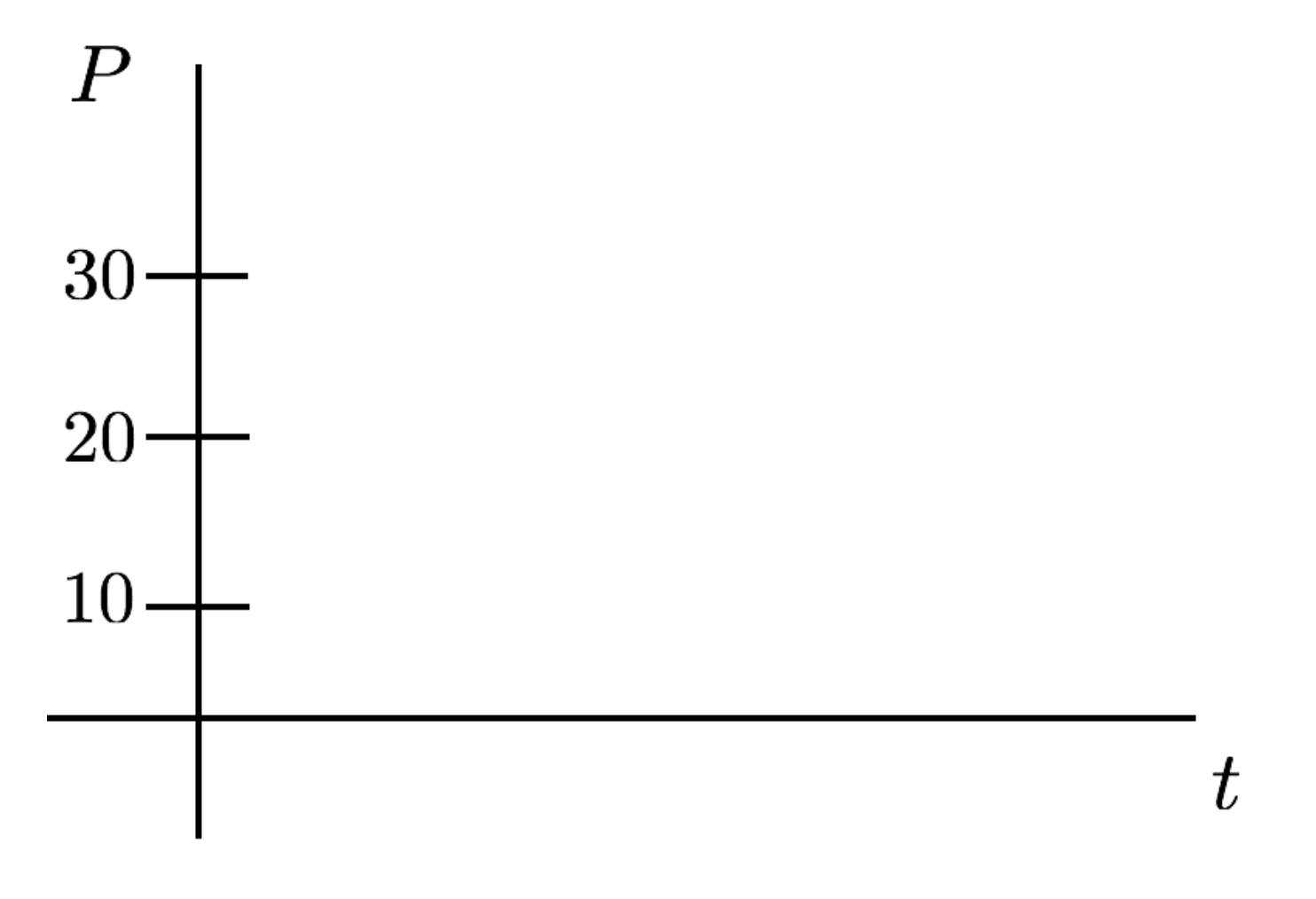
Question 2:
Given these assumptions for a certain lake containing fish, sketch three possible population versus time graphs: one starting at \(P = 10\), one starting at \(P = 20\), and the third starting at \(P = 30\).
Question 2a:
For your graph starting with \(P = 10\), how does the slope vary as time increases? Explain.
Solution to Question 2a:
Question 2b:
For a set \(P\) value, say \(P = 30\), how do the slopes vary across the three graphs you drew?
Solution to Question 2b:
Question 3:
This situation can also be modeled with a rate of change equation, \[\frac{dP}{dt}=\mbox{something}\].
- What should the “something” be?
- Should the rate of change be stated in terms of just \(P\), just \(t\), or both \(P\) and \(t\)?
- Make a conjecture about the right hand side of the rate of change equation and provide reasons for your conjecture.
Solution to Question 3:
What Exactly is a Differential Equation and What are Solutions?
A differential equation is an equation that relates an unknown function to its derivative(s). Suppose \(y = y(t)\) is some unknown function, then a differential equation, would express the rate of change, \(\frac{dy}{dt}\), in terms of \(y\) and/or \(t\). For example, all of the following are first order differential equations.
\[ \frac{dP}{dt}=kP, \qquad \frac{dy}{dt}=y+2t, \qquad \frac{dy}{dt}=t^2+5, \qquad \frac{dy}{dt}=\frac{6y-2}{ty}, \qquad \frac{dy}{dt}=\frac{y^2-1}{t^2+2t}\]
Given a differential equation for some unknown function, solutions are functions that satisfy the rate change equation.
One way to read the differential equation \(\frac{dy}{dt} = y+2t\) aloud you would say, “dee \(y\) dee \(t\) equals \(y\) plus two times \(t\).” However, this does not relate to the meaning of the solution.
Question 4:
Is the function \(y=1+t\) a solution to the differential equation \(\displaystyle\frac{dy}{dt}=\frac{y^2-1}{t^2+2t}\)? How about the function \(y=1+2t\)? How about \(y = 1\)? Explain your reasoning.
Solution to Question 4:
Question 5:
Is the function \(y=t^3+2t\) a solution to the differential equation \(\displaystyle \frac{dy}{dt}=3y^2+2\)? Why or why not?
Solution to Question 5:
Question 6:
Determine all of the functions that satisfy the rate of change equation \(\displaystyle \frac{dP}{dt}=0.3P\).
Solution to Question 6:
Question 7:
Determine all of the solutions to the differential equation \(\displaystyle\frac{dy}{dt}=t^2+5\).
Solution to Question 7:
Introduction to Python
We will be using Python as a tool for experimenting with differential equations. Python is a widely used programming language suited for many purposes and applications such as computational mathematics, data science, and app development. We will create, modify, and run Python code in Jupyter notebooks. No prior programming experience is required to begin working in Python in this (or any future) notebook.
- Python is free and open-source programming language.
- Python has an extensive library of packages with scripts that perform many useful tasks.
- Python is rated as the #2 most in-demand and useful programming languages.
The SymPy Package
Python packages are a collection of modules, functions, data, and/or other code scripts written and openly shared by other users. There are packages to perform many common tasks in mathematics such as plotting graphs, using the number \(\pi\), taking derivatives, and solving equations. This semester, we will frequently use the SymPy package in Python to symbolically differentiate, integrate, and manipulate functions.
Before we can access any files in a package, we must first import the package. Run the code cell below to import the SymPy package with the abbreviation sym.
- We only need to import a package one time during an active Python session.
- We can use the abbreviation
syminstead of the fullsympyto call in functions and modules from the SymPy package.
Symbolic Variables and Functions
Python (like most programming languages) is a very literal language. If we would like to define and store the function \(P = Ae^{kt}\) in Python, we need to be sure Python is reading all the letters and mathematical operations as we intend.
- We might intend some letters such as \(t\) and \(P\) to denote variables.
- Some letters such as \(A\) and \(k\) might denote constant parameters.
- The letter \(e\) denotes the natural exponential number.
The command x, y, z = sympy.symbols('x y z') defines \(x\), \(y\), and \(z\) as variables. We use our abbreviation sym.symbols() for this command. Run the code cell below to create a new symbol t.
t = sym.symbols('t') # Creating t as symbolsSymPy Functions
Next we use functions available within SymPy to create the symbolic function \(P=7e^{0.3t}\).
- We have already defined the symbol
t. - We use the function
sympy.exp()that we abbreviate withsym.exp(). - We must explicitly tell Python how to combine different objects.
- By default, the expression
xyis read as a single object namedxy. - If you want to multiply
xandy, then specify the operation withx * y. - Adding extra spaces helps make the expression easier to read.
- By default, the expression
Run the code cell below to define the exponential function \(P\).
P = 7 * sym.exp(0.3 * t)Printing Output
After running the code cell above, there is no output visible on the screen. The code cell above created the function and stored the function to P. In order to see the output, you need to command Python to print the output to the screen using either print(P) or more simply P.
Run the code cell below to print the function P to the screen.
P # The output for a symbolic function in SymPy is "pretty"Computing Derivatives with SymPy
We now use SymPy to find formulas for derivatives of \(P\) with respect to \(t\).
- The differentiation function is
sympy.diff(f, t, n)finds a formula for the \(n^{\mbox{th}}\) derivative offwith respect to variablet. - If we have already defined function
f, thenf.diff(t, n)can be used in place ofsympy.diff(f, t, n).
sym.diff(P, t, 1) # Differentiate P with respect to tP.diff(t, 1) # Differentiate P with respect to tP.diff(t, 5) # This computes a 5th order derivative.Question 8:
Consider the function \(y = 3\sin{(2x)} - 5 \cos{(2x)}\).
Use SymPy to create a symbolic function and find an expression for \(y''\). Several blank code cells are below to get you started.
Tip
You will first need to create a new symbolic variable x.
Solution to Question 8:
Integration with SymPy
SymPy has an integrals module with lots of built-in functions for computing indefinite and definite integrals as well as common integral transforms (such as Laplace and Fourier transforms).
- The function
sympy.integrate([expr], t)finds an antiderivative (with constant of integration \(C=0\)) of the expression with respect tot. - If we have already stored the expression to the function
f, we can also use the commandf.integrate(t). - To evaluate a definite integral \(\int_a^b f(t) \, dt\), use
sympy.integrate(f, (t, a, b))
We show some examples below. Feel free to experiment!
Caution
The output of sympy.integrate([expr], t) is not the infinite family of all possible antiderivatives. The output is the antiderivative with constant of integration \(C=0\).
t, k = sym.symbols('t, k') # Creating t and k as symbols# Note that indefinite integrals do not include the constant of integration
sym.integrate(t**2 + k, t) # Determines an antiderivative of the function $t^2+k$ with respect to tsym.integrate(t**2 + k, k) # Integrates with respect to ksym.integrate(t**2 + k, (t, 0, 1)) # A definite integral, with respect to t, from 0 to 1sym.integrate(t**2 + k, (t, 0, 1)) # A definite integral, with respect to t, from 0 to 1Question 9:
Consider the differential equation \[ \frac{dQ}{dp} = 2\cos{(3p)}-p^3. \]
Use SymPy find all solutions to the differential equation. Several blank code cells are below to get you started, but students should feel free to make more as needed as well as adding Markdown cells for notes.
Tip
You will first need to create a new symbolic variable p.
Solution to Question 9:
Creative Commons License Information

Exploring Differential Equations by Adam Spiegler is licensed under a Creative Commons Attribution-NonCommercial-ShareAlike 4.0 International License.
Based on a work at https://github.com/CU-Denver-MathStats-OER/ODEs and original content created by Rasmussen, C., Keene, K. A., Dunmyre, J., & Fortune, N. (2018). Inquiry oriented differential equations: Course materials. Available at https://iode.sdsu.edu.