1.2: Slope Fields

Reading: Notes on Diffy Q’s Section 1.2

Plotting a Differential Equation

A slope field is a graphical representation of a rate of change equation. Given a rate of change equation, if we plug in particular values of \((t,y)\) then \(\dfrac{dy}{dt}\) tells you the slope of the tangent vector to the solution at that point.

For example, consider the rate of change equation \(\dfrac{dy}{dt}=\dfrac{t^2y}{4}\).

At the point \((1, 4)\), the value of \(\dfrac{dy}{dt}\) is \(\dfrac{dy}{dt}=\dfrac{(1)^2(4)}{4} =1\).
Thus, the slope field for this equation would show a vector at the point \((1, 4)\) with slope \(1\).

A slope field depicts the exact slope of many such vectors, where we take each vector to be uniform length. Slope fields are useful because they provide a graphical approach for obtaining qualitatively correct graphs of the functions that satisfy a differential equation.

Question 1:

Compute the slope of the solution to \[\dfrac{dy}{dt}= \dfrac{t^2y}{4}\] passing through each of the given points.

\((2,-2)\)
\((0, -1)\)
\((-2,2)\)
\((-3,-2)\)

Solution to Question 1:

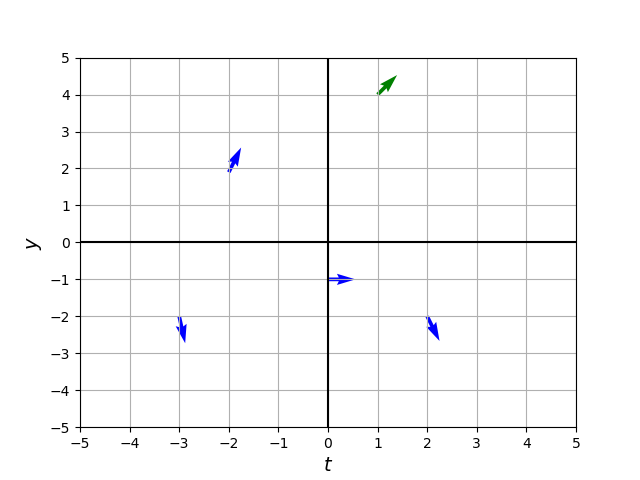
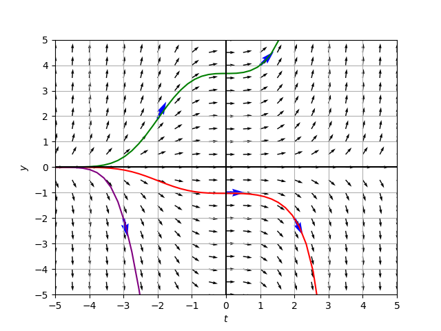
Slope Field for Question 1

The figure on the left shows the corresponding vectors at the points \((1,4)\), \((2,-2)\), \((0, -1)\), \((-2,2)\), and \((-3,-2)\).
The figure on the right gives a more complete slope field with several solutions added.
See the Appendix for the code used to generate the figures below.

A More Complete Slope Fields with Solutions

Question 2:

Describe the “long-run behavior” of the solution to \(\dfrac{dy}{dt}= \dfrac{t^2y}{4}\) that to passes through the given point.

\(y=-1\) when \(t=0\)
\(y(-4) = 1\)
\((2, 0)\)

Solution to Question 2:

Question 3:

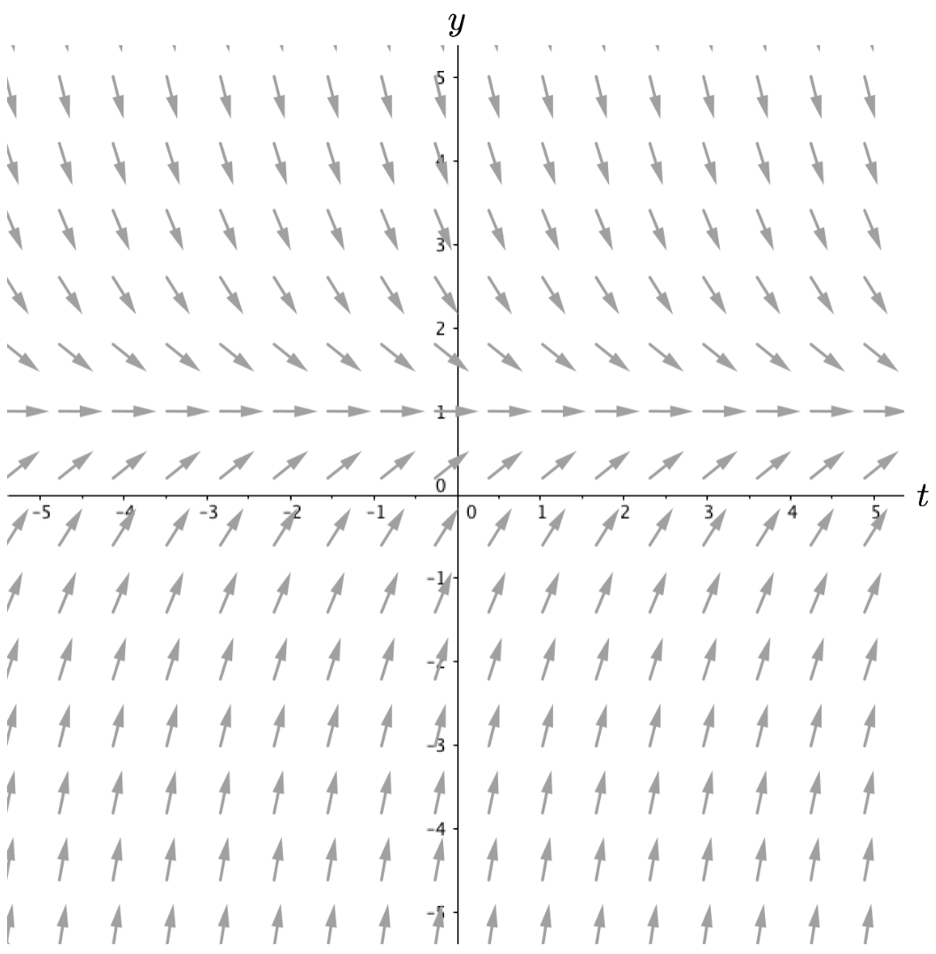
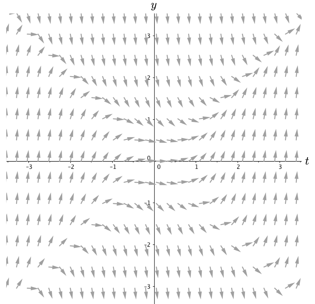
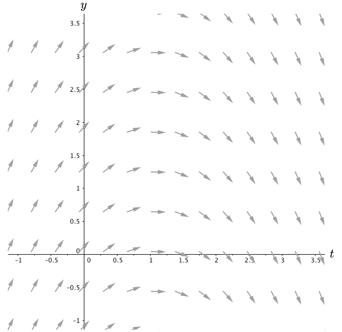
Below are seven differential equations and three different slope fields. Without using technology, identify which differential equation is the best match for each slope field (thus you will have four rate of change equations left over). Explain your reasoning.

\[ \text{(i) } \frac{dy}{dt}=t-1 \quad \text{(ii) } \frac{dy}{dt}=1-y^2 \quad \text{(iii) } \frac{dy}{dt}=y^2-t^2 \quad \text{(iv) } \frac{dy}{dt}=1-y \]

\[ \text{(v) } \frac{dy}{dt}=t^2-y^2 \quad \text{(vi) } \frac{dy}{dt}=1-t \quad \text{(vii) } \frac{dy}{dt}=9t^2-y^2 \]

Slope Field 1	Slope Field 2	Slope Field 3

Solution to Question 3:

Slope field 1 matches equation ??
Slope field 2 matches equation ??
Slope field 3 matches equation ??

Question 4:

For each of the slope fields in Question 3, sketch in graphs of several different qualitatively correct solutions. Do not use any technology to answer this question.

Solution to Question 4:

Sketch your answers on the slope fields above.

Plotting Slope Fields in Python

To create a slope field we can follow the following routine:

Pick a point \((t, y)\) and evaluate the differential equation \(\frac{dy}{dt}\) at that point.
Draw a line segment (of uniform length) with slope \(m=\frac{dy}{dt}\) at the point \((t, y)\).
Repeat many times.

We will use a function named slope_field() whose code is found in the module ode_tools.py that is saved in GitHub.

Loading `ode_tools` from GitHub

Run the code cell below to load the ode_tools module stored in GitHub.
You will only need to run this code cell one time during an active session.
The code cell below will take a couple of seconds to run. You can ignore the output while the code is running.

!pip install git+https://github.com/CU-Denver-MathStats-OER/ODEs
from IPython.display import clear_output
clear_output()

Importing the `slope_field()` Function

Next, import the slope_field() function from the ode_tools module. You will only need to run this command one time during an active session.

from utils.ode_tools import slope_field  # Only need to import one time.

Importing Packages

We need to import two additional use packages in order to plot slope fields with the slope_field() function:

NumPy is a package that is convenient for working with multidimensional arrays (such as vectors and matrices). See NumPy help documentation.
Matplotlib is a package useful for creating static, animated, and interactive visualizations. See Matplotlib help documentation.
- The pyplot subpackage in matplotlib that is a great tool in computational math. See pyplot help documentation.
You only need to import each package one time during an active session.

import numpy as np
import matplotlib.pyplot as plt

Plotting Slope Fields with `slope_field()`

After importing the the packages above, we are ready to create a plot for the slope field of \(\dfrac{dy}{dt}=\dfrac{t^2y}{4}\).

Define arrays t and y to set up the grid where each vector will be plotted. The function np.linspace(initial, end, number) creates an array of number evenly spaced values between initial and end.
Define the differential equation diffeq(t, y).
Generate the slope field with the command slope_field(t, y, diffeq).

Tip

See Quick Reference Guide on How to Use Python Functions for Chapter 1 for more detailed instructions.

# Set up the grid where each vector will be plotted
t = np.linspace(-5, 5, 21)  # picks 21 evenly spaced values between t=-5 and t=5
y = np.linspace(-5, 5, 21)  # picks 21 evenly spaced values between y=-5 and y=5

# Setup the differential equation
def diffeq(t, y):  # t is independent variable and y is dependent variable
    return 0.25 * t**2 * y  # enter the formula for dy/dt

# Run the slope field plotter
slope_field(t, y, diffeq)

Plotting a Different Slope Field

Next we use slope_field() to generate a plot of the slope corresponding to

\[\color{dodgerblue}{\frac{dx}{dq} = 4q^2 - x^2}.\]

We initially choose to plot the slope field over \(-5 \leq q \leq 5\) and \(-5 \leq x \leq 5\). Note when defining diffeq and using the slope_field() function we can change the letters for the independent and dependent variables to \(q\) and \(x\), respectively.

# np.linspace(initial, end, number_values)
q = np.linspace(-5, 5, 21)  # pick 21 values from q=-5 to q=5
x = np.linspace(-5, 5, 21)  # pick 21 values from x=-5 to x=5

# Define a new differential equation
def diffeq(q, x):  # q and x are independent and dependent variables
    return 4 * q**2 - x**2  # formula for dx/dq

Running `slope_field()`

Now that we have defined the differential equation and indicated where the vectors will be plotted, we can generate a new slope field using slope_field(). The code below also changes the color of the vectors from the default color (black) to green.

slope_field(q, x, diffeq, color='green')

Question 5:

Plot each of the four differential equations whose slope fields were not plotted in Question 3.

Solution to Question 5:

Replace each ?? in each of the four code cells below to plot each slope field.

# plot missing slope field 1

# Define points where vectors will be plotted
t = np.linspace(??, ??, ??)  # Independent variable, np.linspace(initial, end, number_values)
y = np.linspace(??, ??, ??)  # Dependent variable, np.linspace(initial, end, number_values)

# Define the differential equation
def diffeq(t, y):  # t is independent variable and y is dependent variable
    return ??  # enter the formula for dy/dt

# Run the slope field plotter
slope_field(t, y, diffeq)

# plot missing slope field 2

# Define points where vectors will be plotted
t = np.linspace(??, ??, ??)  # Independent variable, np.linspace(initial, end, number_values)
y = np.linspace(??, ??, ??)  # Dependent variable, np.linspace(initial, end, number_values)

# Define the differential equation
def diffeq(t, y):  # t is independent variable and y is dependent variable
    return ??  # enter the formula for dy/dt

# Run the slope field plotter
slope_field(t, y, diffeq)

# plot missing slope field 3

# Define points where vectors will be plotted
t = np.linspace(??, ??, ??)  # Independent variable, np.linspace(initial, end, number_values)
y = np.linspace(??, ??, ??)  # Dependent variable, np.linspace(initial, end, number_values)

# Define the differential equation
def diffeq(t, y):  # t is independent variable and y is dependent variable
    return ??  # enter the formula for dy/dt

# Run the slope field plotter
slope_field(t, y, diffeq)

# plot missing slope field 4

# Define points where vectors will be plotted
t = np.linspace(??, ??, ??)  # Independent variable, np.linspace(initial, end, number_values)
y = np.linspace(??, ??, ??)  # Dependent variable, np.linspace(initial, end, number_values)

# Define the differential equation
def diffeq(t, y):  # t is independent variable and y is dependent variable
    return ??  # enter the formula for dy/dt

# Run the slope field plotter
slope_field(t, y, diffeq)

Adding a Solution to a Slope Field

Importing `plot_sol()`

We have seen that slope fields are useful for sketching graphs to approximate solutions that pass through certain points. The arrows should be approximately tangent to the curve we sketch. In addition to the slope_field() function we used earlier, the ode_tools module defines other functions we will use this semester. We next import the function plot_sol() to plot a slope field as well as the solution that passes through a given point.

from utils.ode_tools import plot_sol  # Only need to import the function once

Using the `plot_sol()` Function

After importing the the plot_sol() function from ode_tools and the NumPy and Matplotlib packages, we are ready to create a plot for the slope field of \(\dfrac{dy}{dt}=\dfrac{t^2y}{4}\) with the graph of the solution through the point \((-2,2)\).

Use np.linspace() to define arrays t and y to set up the grid where each vector will be plotted.
Define the differential equation diffeq(t, y).
Define an initial condition \((t_0, y_0)\).
- The initial value of \(y\) is stored in the variable named y0.
Generate the slope field with the command plot_sol(t, y, diffeq, t0, y0).

Tip

See Quick Reference Guide on How to Use Python Functions for Chapter 1 for more detailed instructions.

#from utils.ode_tools import plot_sol  # Only need to import the function once

# Define points where vectors will be plotted
t = np.linspace(-5, 5, 21)  
x = np.linspace(-5, 5, 21)

# Define the differential equation
def diffeq(t, y):  # t is independent variable and y is dependent variable
    return 0.25 * t**2 * y  # enter the formula for dy/dt

# Enter t0, the initial value of t
# Enter y0, the value of y at t0
t0 = -2
y0 = 2

# Run the function to create a plot
plot_sol(t, y, diffeq, t0, y0)

Question 6:

Use the plot_sol() function to create a plot of the slope field and solution passing through the given point.

\[\color{dodgerblue}{\frac{dx}{dq} = 4q^2 - x^2, \qquad x(-2)=3}.\]

Solution to Question 6:

Complete the code block below.

#from utils.ode_tools import plot_sol  # Only need to import the function once

# Define points where vectors will be plotted
q = np.linspace(??, ??, ??)  
x = np.linspace(??, ??, ??)  

# Define the differential equation
def diffeq(q, x):  # q is independent variable and x is dependent variable
    return ??  # enter the formula for dx/dq

# Enter q0, the initial value of q
# Enter x0, the value of x at q0
q0 = ??
x0 = ??

# Run the function to create a plot
plot_sol(q, x, diffeq, q0, x0)

Appendix: Code for Plots After Question 1

The code cells below generate the figure illustrating the solution to Question 1.

# import required packages
import matplotlib.pyplot as plt
import numpy as np
from scipy.integrate import odeint, solve_ivp  # numerical ode solver

# Plot 5 vectors in slope field
plt.quiver(1, 4, 1, 1, color = 'green')  # Plot vector at (1,4) with slope dy/dt = 1/1 = 1 
plt.quiver(2, -2, 1, -2, color = 'blue')  # Plot vector at (2,-2) with slope dy/dt = -2/1 = -2  
plt.quiver(-3, -2, 1, -4.5, color = 'blue')  # Plot vector at (-3,-2) with slope dy/dt = -4.5/1 = -4.5 
plt.quiver(-2, 1.9, 1, 2, color = 'blue')  # Plot vector at (-2,2) with slope dy/dt = 2/1 = 2 
plt.quiver(0, -1, 1, 0, color = 'blue')  # Plot vector at (0,-1) with slope dy/dt = 0/1 = 0 

# Set limits on horizontal and vertical axes
plt.xlim([-5, 5])
plt.ylim([-5, 5])

# Label axes
plt.xlabel(r"$t$", fontsize=14)
plt.ylabel(r"$y$", fontsize=14)

# Add a grid and axes to plot
plt.xticks(np.linspace(-5,5,11))
plt.yticks(np.linspace(-5,5,11))
plt.grid(True, which='both')
plt.axvline(x=0, color='black')
plt.axhline(y=0, color='black')

plt.show()

# Solutions to diff eq
t = np.linspace(-5, 5, 50)  # time interval for solution plots
y0 = np.array([0.00011, -0.000030732613, -0.000568])  # initial conditions when t=-5

# Define diff eq
def model(y, t):  # t is independent variable and y is dependent variable
    dydt = 0.25 * t**2 * y  # enter the formula for dy/dt
    return dydt

# solve the IVP 1
sol1 = odeint(model, y0[0], t)
# solve the IVP 2
sol2 = odeint(model, y0[1], t)
# solve the IVP 3
sol3 = odeint(model, y0[2], t)

# Plot the 3 solutions
plt.plot(t, sol1, color='green', linestyle='dashed', linewidth=1.0)
plt.plot(t, sol2, color='red', linestyle='dashed', linewidth=1.0)
plt.plot(t, sol3, color='purple', linestyle='dashed', linewidth=1.0)

# Plot vectors 5 vectors
plt.quiver(1, 4, 1, 1, color = 'green')  # plots vector at (1,4) with slope 1/1 = 1 
plt.quiver(2, -2, 1, -2, color = 'blue')  # plots vector at (2,-2) with slope -2/1 = -2
plt.quiver(-3, -2, 1, -4.5, color = 'blue')  # plots vector at (-3,-2) with slope -4.5/1 = -4.5
plt.quiver(-2, 1.9, 1, 2, color = 'blue')  # plots vector at (-2,1.9) with slope 2/1 = 2
plt.quiver(0, -1, 1, 0, color = 'blue')  # plots vector at (0,-1) with slope 0/1 = 0

# Set limits on x and y axes
plt.xlim([-5, 5])
plt.ylim([-5, 5])

# Label axes
plt.xlabel(r"$t$", fontsize=14)
plt.ylabel(r"$y$", fontsize=14)

# Add a grid and axes to plot
plt.xticks(np.linspace(-5,5,11))
plt.yticks(np.linspace(-5,5,11))
plt.grid(True, which='both')
plt.axvline(x=0, color='black')
plt.axhline(y=0, color='black')

plt.show()

fig = plt.figure()

# Plot a more complete slope field
X, Y = np.meshgrid(np.linspace(-5, 5, 21), np.linspace(-5, 5, 21))
U = 1.0
V = 0.25 * Y * X ** 2
# Normalize arrows
N = np.sqrt(U ** 2 + V ** 2)
U = U / N
V = V / N
plt.quiver(X, Y, U, V, angles="xy")

# Plot 3 solutions
plt.plot(t, sol1, color='green', linewidth=1.5)
plt.plot(t, sol2, color='red', linewidth=1.5)
plt.plot(t, sol3, color='purple', linewidth=1.5)


# Plot 5 vectors
plt.quiver(1, 4, 1, 1, color = 'blue')  # plots vector at (1,4) with slope 1/1 = 1 
plt.quiver(2, -2, 1, -2, color = 'blue')  # plots vector at (2,-2) with slope -2/1 = -2
plt.quiver(-3, -2, 1, -4.5, color = 'blue')  # plots vector at (-3,-2) with slope -4.5/1 = -4.5
plt.quiver(-2, 1.9, 1, 2, color = 'blue')  # plots vector at (-2,1.9) with slope 2/1 = 2
plt.quiver(0, -1, 1, 0, color = 'blue')  # plots vector at (0,-1) with slope 0/1 = 0

# Add a grid and axes to plot
plt.xticks(np.linspace(-5,5,11))
plt.yticks(np.linspace(-5,5,11))
plt.grid(True, which='both')
plt.axvline(x=0, color='black')
plt.axhline(y=0, color='black')

plt.xlim([-5, 5])
plt.ylim([-5, 5])
plt.xlabel(r"$t$")
plt.ylabel(r"$y$")

Creative Commons License Information

Exploring Differential Equations by Adam Spiegler is licensed under a Creative Commons Attribution-NonCommercial-ShareAlike 4.0 International License.
Based on a work at https://github.com/CU-Denver-MathStats-OER/ODEs and original content created by Rasmussen, C., Keene, K. A., Dunmyre, J., & Fortune, N. (2018). Inquiry oriented differential equations: Course materials. Available at https://iode.sdsu.edu.

Plotting a Differential Equation

Question 1:

Solution to Question 1:

Slope Field for Question 1

Question 2:

Solution to Question 2:

Question 3:

Solution to Question 3:

Question 4:

Solution to Question 4:

Plotting Slope Fields in Python

Loading ode_tools from GitHub

Importing the slope_field() Function

Importing Packages

Plotting Slope Fields with slope_field()

Plotting a Different Slope Field

Running slope_field()

Question 5:

Solution to Question 5:

Adding a Solution to a Slope Field

Importing plot_sol()

Using the plot_sol() Function

Question 6:

Solution to Question 6:

Appendix: Code for Plots After Question 1

Creative Commons License Information

Loading `ode_tools` from GitHub

Importing the `slope_field()` Function

Plotting Slope Fields with `slope_field()`

Running `slope_field()`

Importing `plot_sol()`

Using the `plot_sol()` Function