!pip install git+https://github.com/CU-Denver-MathStats-OER/ODEs
from IPython.display import clear_output
clear_output()3.5: Stability of Equilibria
![]()
Reading: Notes on Diffy Q’s Section 3.5
Initial Conditions of Systems
Question 1:
Recall model of the bacteria populations in Colony 1 and Colony 2 given by system of differential equations
\[\begin{align} \frac{dx}{dt} &= 3x+10y \\ \frac{dy}{dt} &= -2y \end{align}\]
We previously found the general solution for this system, which can be expressed as
\[\begin{align} x(t)&= C_1e^{3t} + C_2 e^{-2t} \\ y(t)&= - \frac{1}{2} C_2 e^{-2t} \\ \end{align}\]
Question 1a:
Give the solutions if in addition we have the initial condition \((x(0),y(0))= (3,0)\).
Solution to Question 1a:
Question 1b:
Give the solutions if in addition we have another initial condition \((x(0),y(0))= (2,-1)\).
Solution to Question 1b:
Question 1c:
Sketch the graphs (in the phase plane) of the solution with initial condition \((x(0),y(0))= (3,0)\) and the solution with initial condition \((x(0),y(0))= (2,-1)\).
Tip
You may sketch by hand (probably quicker!) or using the code cells below.
Solution to Question 1c:
Loading ode_tools from GitHub
- Run the code cell below to load the most up to date modules stored in GitHub.
- You will only need to run this code cell one time during an active session.
Importing phase_portrait from ode_tools Module
from utils.ode_tools import phase_portrait # Only need to import one time.Plotting Solutions in the Phase Plane
import numpy as np

# Set viewing window

x = np.linspace(-5.0, 5.0, 23)  # x is horizontal axis
y = np.linspace(-5.0, 5.0, 23)  # y is vertical axis

#############################################
# Enter the system of differential equations
#############################################

def f(Y, t):
    x, y = Y
    return [3*x + 10*y ,  # diff eq for dx/dt
            -2*y]  # # diff eq for dy/dt
import matplotlib.pyplot as plt # import plotting package
# Plots a phase portrait
phase_portrait(x, y, f)
# line through (3,0)
plt.plot(x, ??, linewidth=2, color='b') # replace ?? with an expression
# line through (2, -1)
plt.plot(x, ??, linewidth=2, color='r') # replace ?? with an expressionQuestion 1d:
Using your graph in the previous question, make a rough sketch of the solution corresponding to the initial conditions \((x(0),y(0))= (1,1)\) and \((x(0),y(0))= (1,-1)\).
Solution to Question 1d:
Eigenvectors
For the system
\[\begin{bmatrix} x' \\ y' \end{bmatrix} = \begin{bmatrix} 3 & 10 \\ 0 & -2 \end{bmatrix} \begin{bmatrix} x\\ y \end{bmatrix}, \]
\(\mathbf{v}_1=\langle 3, 0 \rangle\) is an eigenvector corresponding to the eigenvalue \(r_1 = 3\) and \(\mathbf{v}_2=\langle -2, 1 \rangle\) is an eigenvector of \(r_2=-2\). From phase plane graph in Question 1d, we see that any solution that starts on the line passing through the eigenvector:
- \(\mathbf{v}_1=\langle 3, 0 \rangle\) points directly away from the equilibrium at the origin.
- \(\mathbf{v}_2=\langle 2, -1 \rangle\) points directly towards the origin.
- The sign of the eigenvalue determines whether solutions move towards or away from the equilibrium.
In general, \(\mathbf{v}\) is an eigenvector for the eigenvalue \(\lambda\) of a square matrix \(A\) if and only if
\[A \mathbf{v} = \lambda \mathbf{v}.\]
Eigenvectors in Sympy
import sympy as sym

M = sym.Matrix([[3, 10],
           [0, -2]])

M.eigenvects()
Expressing Solutions in Vector Form
Using the eigenvectors we can express the solutions in vector form:
\[\begin{align} \begin{bmatrix} x(t) \\ y(t) \end{bmatrix} &= C_1e^{r_1t} \mathbf{v}_1+ C_2 e^{r_2t} \mathbf{v}_2 \\ \\ \color{dodgerblue}{\begin{bmatrix} x(t) \\ y(t) \end{bmatrix}} & \color{dodgerblue}{= C_1e^{3t} \begin{bmatrix} 3 \\ 0 \end{bmatrix} + C_1e^{-2t} \begin{bmatrix} -2 \\ 1 \end{bmatrix}} \end{align}\]
The vector form of the solution above is equivalent to solutions we obtained earlier:
\[\begin{bmatrix} x(t) \\ y(t) \end{bmatrix} = \begin{bmatrix} 3C_1e^{3t} & - & 2C_2e^{-2t} \\ & & C_2e^{-2t} \end{bmatrix} \quad \mbox{so we have} \quad x(t) = B_1e^{3t}+B_2e^{-2t} \mbox{ and } y(t) = - \frac{1}{2}B_2e^{-2t}.\]
Question 2:
Consider the system of differential equations:
\[\begin{bmatrix} x'\\ y' \end{bmatrix} = \begin{bmatrix} 1 & 3 \\ 4 & 5 \end{bmatrix} \begin{bmatrix} x\\ y \end{bmatrix}\]
Find the eigenvalues and eigenvectors for the system, and give the general solution in vector form. Then make a sketch of several solutions to this system in the phase plane by hand.
Tip
Feel free to use code cells to help find eigenvalues and eigenvectors.
Solution to Question 2:
Eigenvalues and Solutions in the Phase Plane
Question 3:
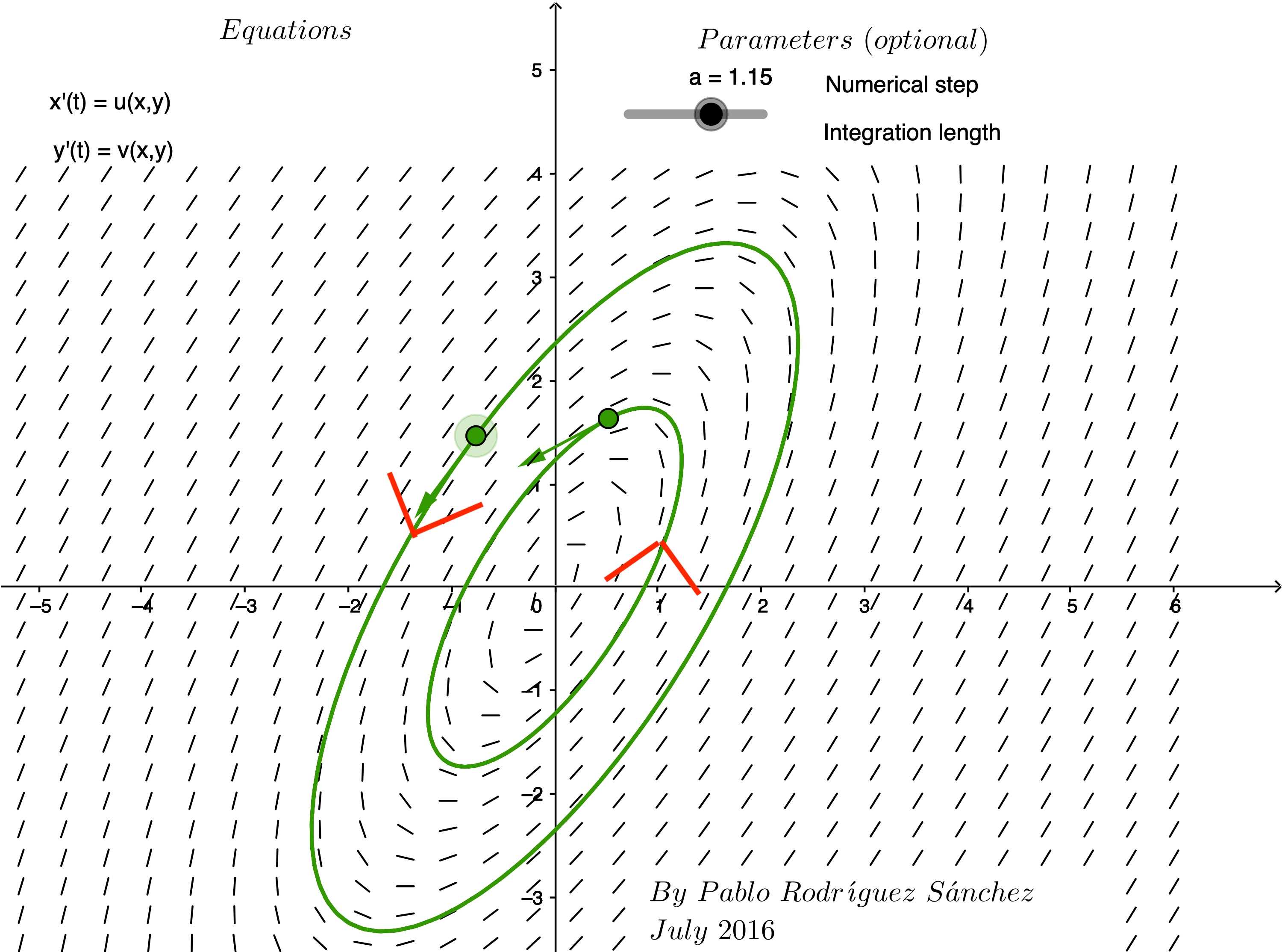
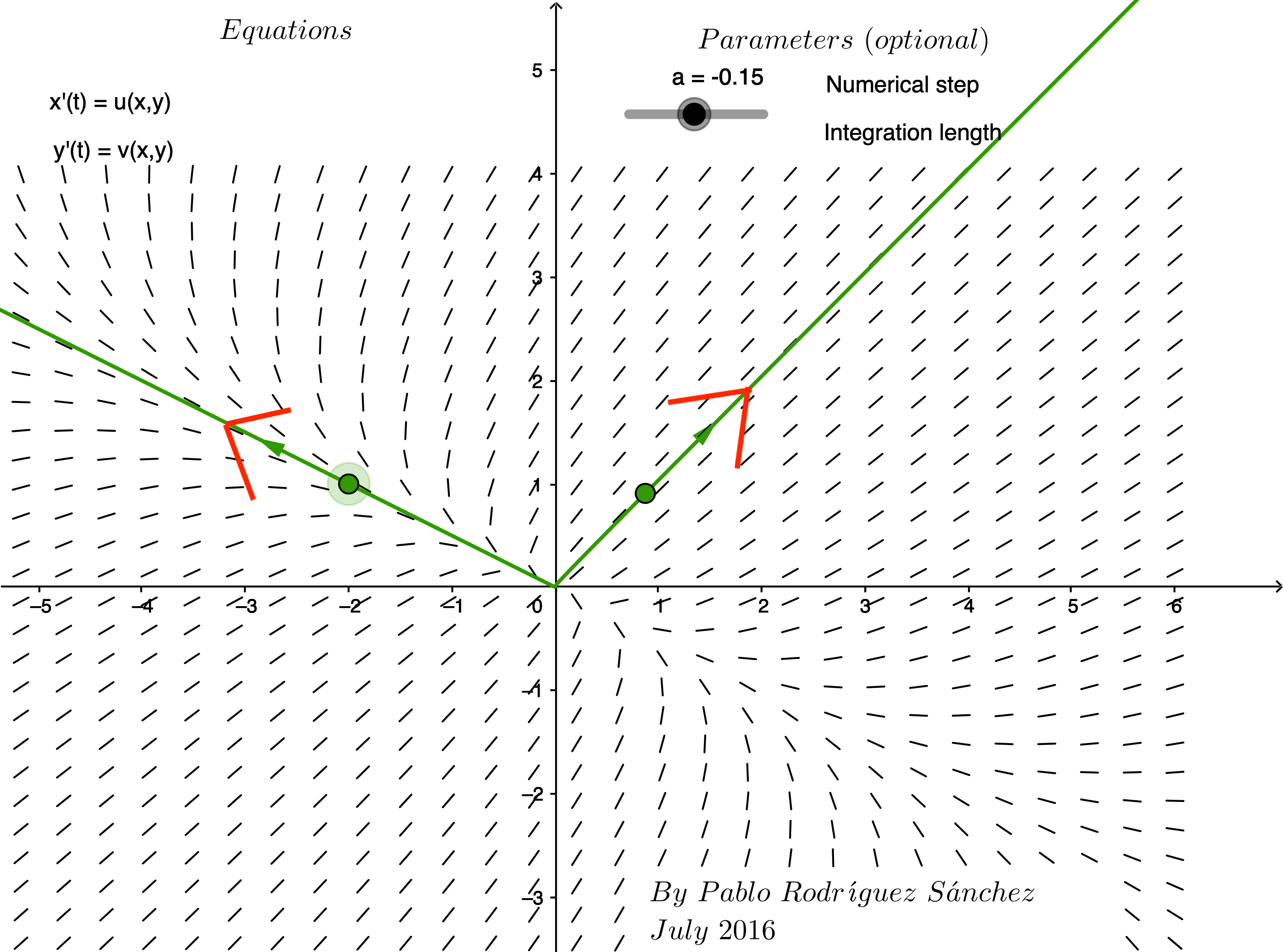
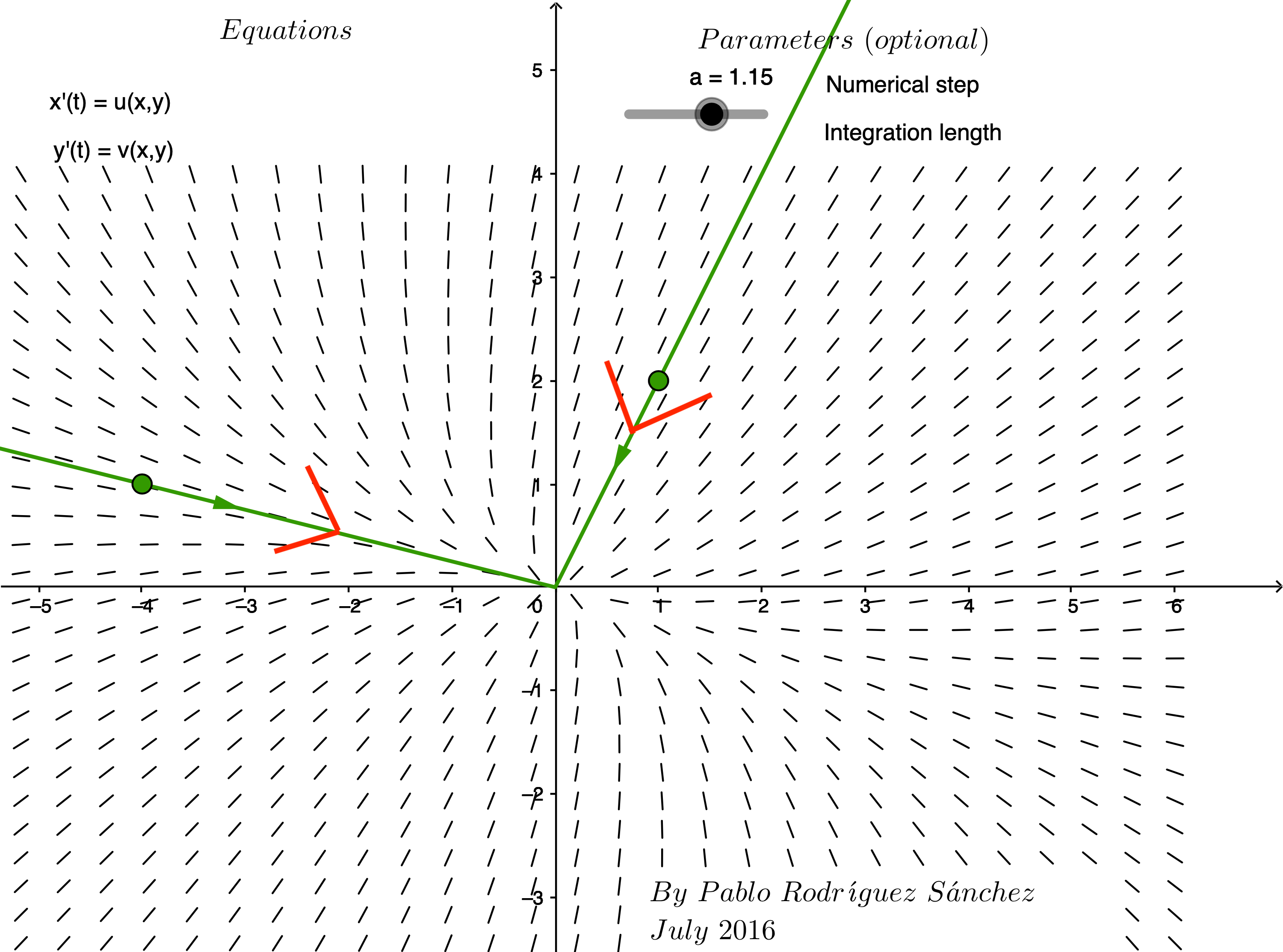
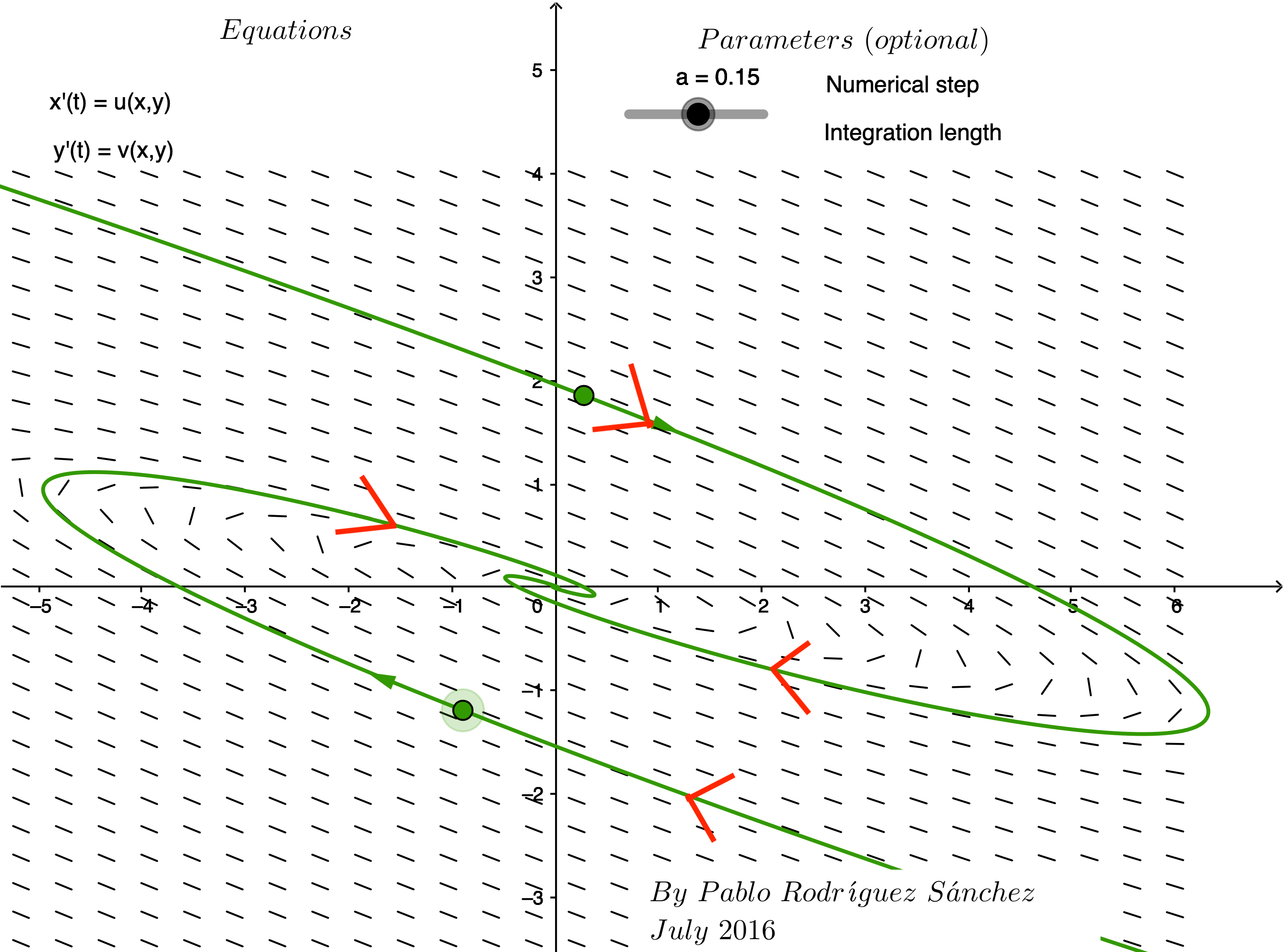
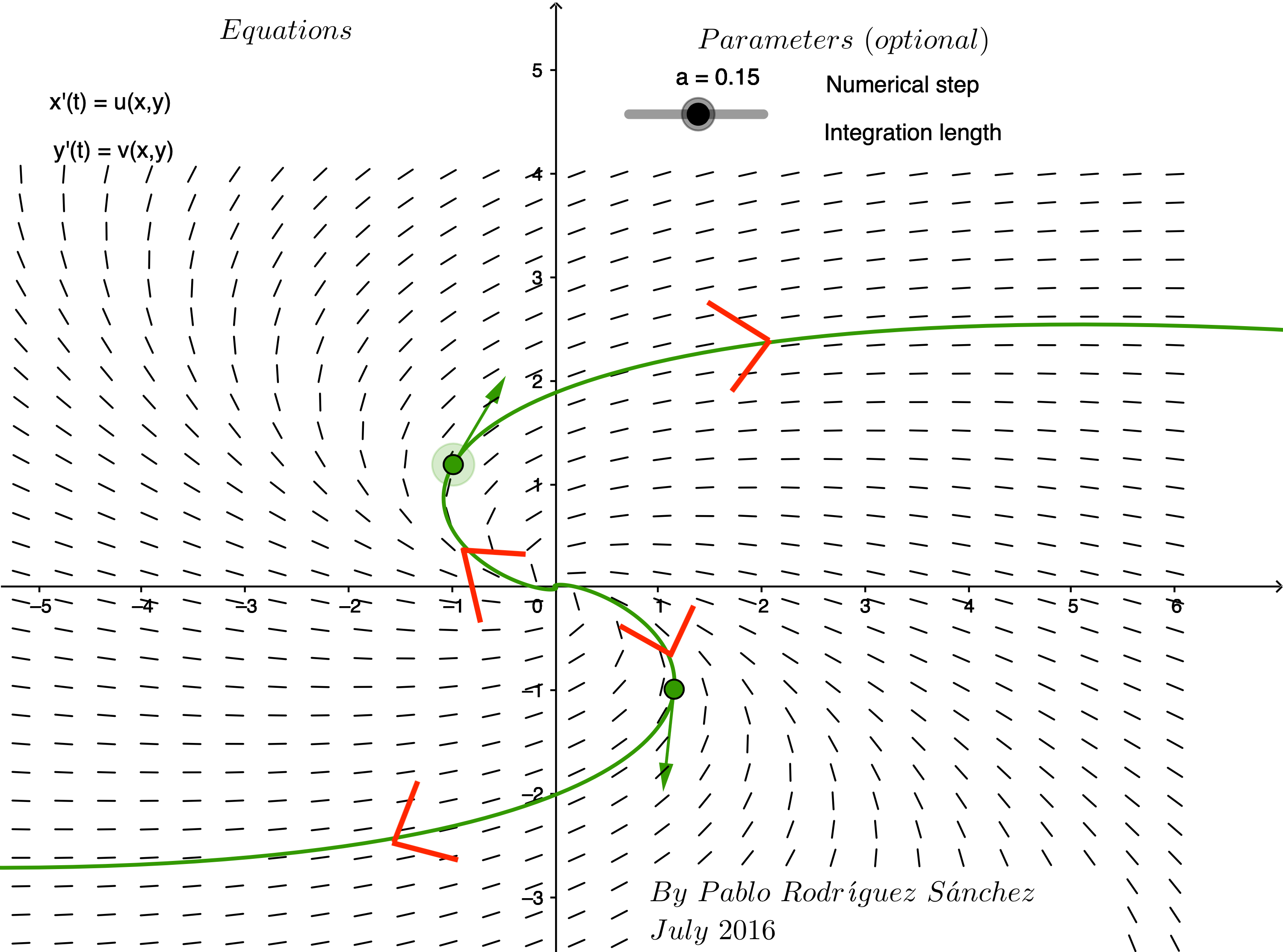
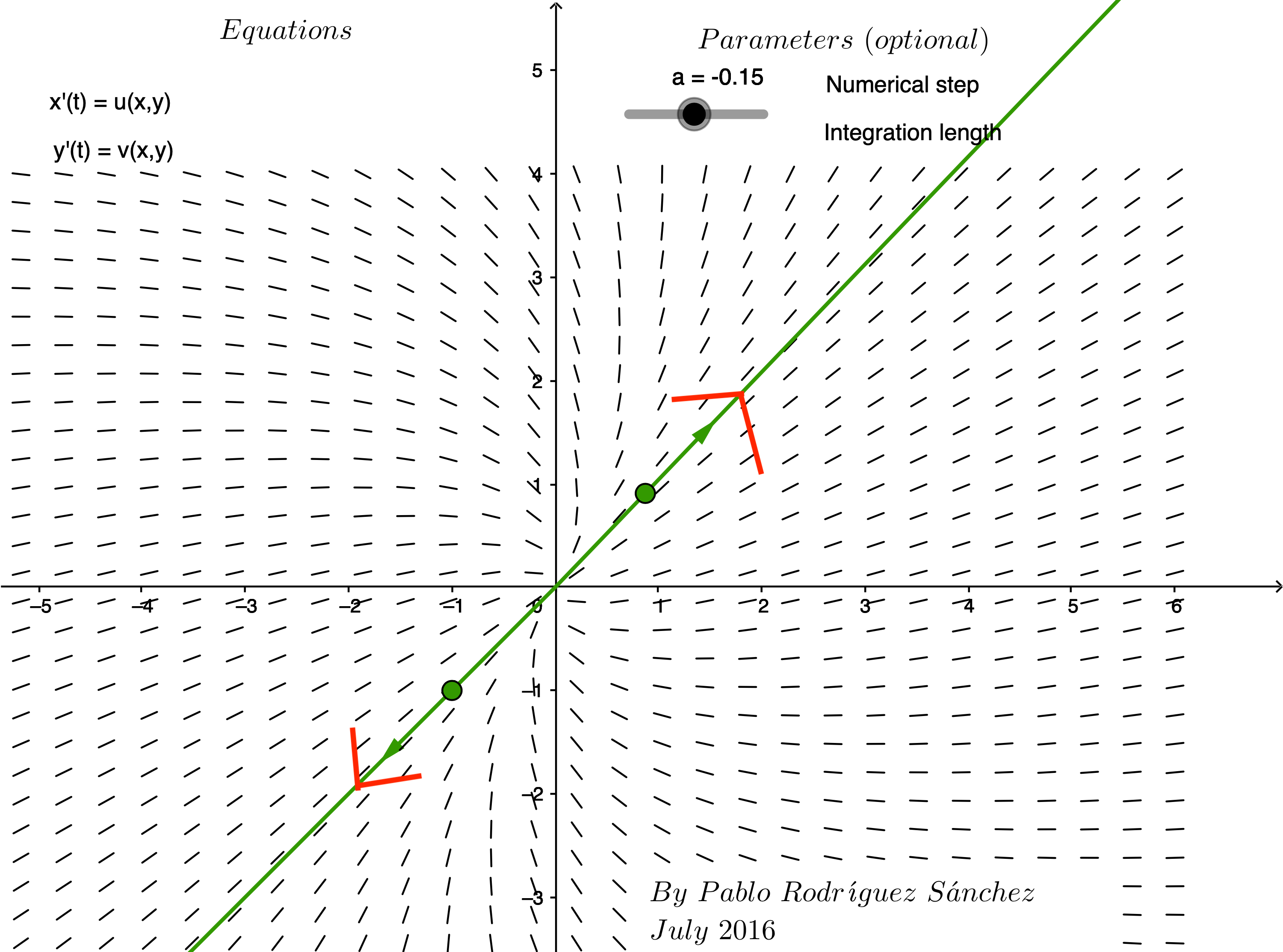
Match the vector fields labeled A-F with a system of differential equations whose matrix of coefficients has the given eigenvalues.
| Eigenvalues of matrix of coefficients | Label of corresponding phase plane |
|---|---|
| \[\lambda_1 = 4 \mbox{ and } \lambda_2=1\] | Enter letter of matching graph |
| \[\lambda_1 = -4 \mbox{ and } \lambda_2=-2\] | Enter letter of matching graph |
| \[\lambda = 9 \mbox{ repeated } \] | Enter letter of matching graph |
| \[\lambda = \pm 2i \] | Enter letter of matching graph |
| \[\lambda = 3 \pm 2i \] | Enter letter of matching graph |
| \[\lambda = -3 \pm 2i \] | Enter letter of matching graph |
| A | B |
|---|---|
 |
 |
| C | D |
|---|---|
 |
 |
| E | F |
|---|---|
 |
 |
Solution to Question 3:
Express your answers by completing the table above.
Stability of the Equilibrium
Question 4:
Based on your answers in Question 3, explain how the eigenvalues can be used to determine whether the equilibrium at the origin is stable or unstable? What happens when the matrix of coefficients has complex eigenvalues?
Solution to Question 4:
Creative Commons License Information

Exploring Differential Equations by Adam Spiegler is licensed under a Creative Commons Attribution-NonCommercial-ShareAlike 4.0 International License.
Based on a work at https://github.com/CU-Denver-MathStats-OER/ODEs and original content created by Rasmussen, C., Keene, K. A., Dunmyre, J., & Fortune, N. (2018). Inquiry oriented differential equations: Course materials. Available at https://iode.sdsu.edu.