!pip install git+https://github.com/CU-Denver-MathStats-OER/ODEs
from IPython.display import clear_output
clear_output()2.2: Homogeneous Equations
![]()
Reading: Notes on Diffy Q’s Section 2.2 Part 2 (complex roots)
Solving the Homogeneous Equations
A second order linear differential equation with constant coefficients has the form
\[\color{dodgerblue}{a \frac{d^2x}{dt^2}+b\frac{dx}{dt}+cx=}{\color{tomato}{f(t)}}\]
where \(a\), \(b\), and \(c\) are constants and \(f\) is a continuous function of \(t\).
- If \(\color{tomato}{f(t)=0}\), then the equation is called homogeneous.
- If \(\color{tomato}{f(t)\ne 0}\), then the equation is called nonhomogeneous.
Revisiting the Roots of the Characteristic Equation
We have shown that to find solutions to the homogeneous case \(a \dfrac{d^2x}{dt^2}+b\dfrac{dx}{dt}+cx =0\), we can:
- Set up the corresponding characteristic polynomial, \(ar^2+br+c=0\).
- Find solutions \(r=r_1\) and \(r=r_2\) to the characteristic equation.
- Quadratic equations may have real or complex solutions:
- If \(r_1\) and \(r_2\) are distinct real numbers, then the general solution is \(x(t) = C_1e^{r_1t} + C_2e^{r_2t}\).
- If there is one repeated root, \(r_1\), then the general solution is \(x(t) = C_1e^{r_1t} + C_2{\color{tomato}{t}}e^{r_1t}\).
- If the solutions are of the form \(\mathbf{r = \alpha \pm i \beta}\), then what?
Question 1:
Let \(\displaystyle f(t)=e^{i \beta t}\) and answer the questions below.
Question 1a:
Find a formula for \(f'\), \(f''\), \(f'''\), \(f^{iv}\), and \(f^{v}\).
Solution to Question 1a:
Question 1b:
Express \(f(t)=e^{i \beta t}\) using as a Taylor series at \(t=0\).
\[f(t) = f(0) + \frac{f'(0)}{1!}t + \frac{f''(0)}{2!} t^2 + \frac{f'''(0)}{3!} t^3 + \frac{f^{iv}(0)}{4!} t^4 + \frac{f^{v}(0)}{5!} t^5 + \ldots\]
Solution to Question 1b:
Question 1c:
Group the real and imaginary parts of the first several terms in the Taylor series together.
Solution to Question 1c:
Question 1d:
Do you recognize these are Taylor series of common functions?
Solution to Question 1d:
Euler’s Formula
The previous question is a proof of Euler’s formula which allows us to write exponentials in polar form,
\[\large \color{dodgerblue}{e^{(\alpha + i \beta) t} = e^{\alpha t} \bigg( \cos{(\beta t)} + i \sin{(\beta t)} \bigg).}\]
Question 2:
If \(z(t)=P(t)+i Q(t)\) is complex solution to a differential equation of the form \(az''+bz'+cz=0\), prove that the real part \(P(t)\) is a solution itself and the imaginary part \(Q(t)\) (not including the \(i\)) is also a solution itself.
Note
The derivative of a complex function is the sum of the derivatives of the real and imaginary parts of the complex function \(z'(t) = P'(t) + i Q'(t)\).
Solution to Question 2:
Question 3:
Find the general solution to the homogeneous differential equation
\[\frac{d^2x}{dt^2}+2 \frac{dx}{dt} + 17x=0\]
Use the results from Question 2 on exponentiation of complex numbers to find the general solution to the differential equation.
Solution to Question 3:
Question 4:
Replace each blank in the cell below with an appropriate formula.
Solution to Question 4:
Fill in solutions below.
General Solution when Roots are Complex
To summarize our results, when solving a homogeneous second order differential with constant coefficients, we can find the zeros of the corresponding characteristic equation. Then
- If \(r_1\) and \(r_2\) are distinct real numbers, then the general solution is
\[\_\_\_\_?\_\_\_\_\]
- If there is one repeated root, \(r_1\), then the general solution is
\[\_\_\_\_?\_\_\_\_\]
- If there are complex solutions of the form \(r = \alpha \pm i \beta\), then the general solution is
\[\_\_\_\_?\_\_\_\_\]
Question 5:
Find a general solution to the differential equation \(\displaystyle 2y''+7y'-4y=0\).
Solution to Question 5:
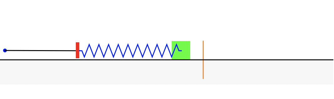
Mass-Spring Oscillator
Imagine we connect an object with mass \(m\) kg to a spring with stiffness coefficient \(k\) kg/sec\(^2\) that is connected to a stationary wall on the other end. We give the mass some initial position \(s_0\) and velocity \(v_0\), and we observe the mechanics of how the mass moves along a surface with friction coefficient \(b\) kg/sec. Such a system is called a mass-spring oscillator or a harmonic oscillator. The position of the mass at time, \(y(t)\), is modeled by the second order differential equation
\[\large {\color{mediumseagreen}{m}}y''+{\color{tomato}{b}}y'+{\color{dodgerblue}{k}}y=0; \qquad y(0)=s_0, \quad y'(0)=v_0.\]
Question 6:
Consider the mass-spring oscillator that has mass \(m=1\) kg, stiffness \(k=4\) kg/sec\(^2\), and damping \(b\) kg/sec. The displacement \(y\) from equilibrium position at time \(t\) seconds satisfies the initial value problem
\[y''+by'+4y=0; \ \ y(0)=1 \ \ y'(0)=0.\]
Question 6a:
Interpret the practical meaning of the initial conditions.
Solution to Question 6a:
Question 6b:
Find the solution if the damping coefficient is \(b=0\) and describe what happens to the mass as \(t \to \infty\).
Solution to Question 6b:
Question 6c:
Find the solution if the damping coefficient is \(b=5\) and describe what happens to the mass as \(t \to \infty\).
Solution to Question 6c:
Question 6d:
Find the solution if the damping coefficient is \(b=4\) and describe what happens to the mass as \(t \to \infty\).
Solution to Question 6d:
Question 6e:
Find the solution if the damping coefficient is \(b=2\) and describe what happens to the mass as \(t \to \infty\).
Solution to Question 6e:
Testing Our Results in the Mass-Spring Lab
We now import a function named damped_harmonic_oscillator() that lives inside a module named mass_spring stored in GitHub.
- See Mass-Spring-Tutorial.ipynb for more detailed instructions.
Importing damped_harmonic_oscillator
- Run the first code cell below to load the most up to date modules stored in GitHub.
- Run the second code cell to import the
damped_harmonic_oscillatorfunction from themass_springmodule
from utils.mass_spring import damped_harmonic_oscillator # Only need to import one time.Running Experiments
Recall the mass-spring system (also called a damped harmonic oscillator) has the following model
\[my''+by'+ky=0; \ \ y(0)=s_0 \ \ y'(0)=v_0.\]
In Question 6 we have:
- \(m=1\),
- \(k=4\),
- and then we condsidered what happens when we change the amount of friction (damping) in the system.
Experiment with the value of \(b\) in the code cell below, and see how changing \(b\) affects the behavior of mass-spring systems.
- Note the animation may take several seconds to complete running.
damped_harmonic_oscillator(m=1,  # mass is 1
                           b=0,  # friction is 0
                           k=4,  # stiffness is 4
                           x0=[1,0])  # initial position and velocity
Running A Side-by-Side Comparison
The function damped_harmonic_comp() will simultaneously run to animations for two different mass-spring systems.
Below we compare an underdampled and overdamped system.
- You first need to import the
damped_harmonic_compfunction frommass_spring. You only need to do this one time in an active sesion. - Set parameters for both systems.
- Run the code cell. I may take up to a minute to run.
- Press the play button.
from utils.mass_spring import damped_harmonic_oscillator_compdamped_harmonic_oscillator_comp(m=[0.2, 0.3], # masses
b=[0.5, 0.1], # frictions
k=[1, 2], # stiffnesses
A=[0, 0], # Amplitudes of forcing
omega=[1, 1], # Frequencies of forcing
x0=[[0.5, 1], [-0.5, -1]], # initial conditions
fps=4, # frames per second
tf=40) # total timeCreative Commons License Information

Exploring Differential Equations by Adam Spiegler is licensed under a Creative Commons Attribution-NonCommercial-ShareAlike 4.0 International License.
Based on a work at https://github.com/CU-Denver-MathStats-OER/ODEs and original content created by Rasmussen, C., Keene, K. A., Dunmyre, J., & Fortune, N. (2018). Inquiry oriented differential equations: Course materials. Available at https://iode.sdsu.edu.