3.2: Phase Plane Portraits

Slope fields are a convenient way to visualize solutions to a single differential equation. For systems of autonomous differential equations the equivalent representation is a vector field often called a phase plane portrait. Similar to a slope field, a phase plane portrait shows a selection of vectors with the correct slope but with a normalized length.

Plotting Phase Plane Portraits with `phase_portrait`

As with slope fields, we typically rely on technology to plot phase plane portraits. The ode_tools module (same file as earlier) includes a function called phase_portrait that will be a nice tool for visualizing solutions to autonomous systems of differential equations.

Loading `ode_tools` from GitHub

Run the code cell below to load the most up to date modules stored in GitHub.
You will only need to run this code cell one time during an active session.

!pip install git+https://github.com/CU-Denver-MathStats-OER/ODEs
from IPython.display import clear_output
clear_output()

Importing the `phase_portrait` Plotting Function

After you followed the instructions above and set your file path, you are now ready to import the phase_portrait function from the ode_tools module.

from utils.ode_tools import phase_portrait  # Only need to import one time.

Defining the System of Differential Equations

Recall the rabbit and fox population model from 14-Introduction-to-Systems.

\[\begin{align} \frac{dR}{dt} &= 3R-1.4RF\\ \frac{dF}{dt} &= -F+0.8RF \end{align}\]

In the code cell below, we choose a window of \(0 \leq R, F \leq 5\) and enter the system of differential equations.

import numpy as np

# Set viewing window
x = np.linspace(0.0, 5.0, 20)  # values for horizontal axis of phase plane
y = np.linspace(0.0, 5.0, 20)  # values for vertical axis of phase plane

# Define the system of differential equations
def f(Y, t):
    x, y = Y
    return [3*x - 1.4*x*y,  # enter formula for diff eq for x
            -y + 0.8*x*y]  # enter formula for diff eq for y

Plotting with `phase_portrait`

# Plots a phase portrait

phase_portrait(x, y, f)

Adding a Solution to a Phase Plane Portrait with `plot_phase_sol`

Let’s add a plot of the solution with initial condition \((R,F)=(2,3)\) to the phase plane portrait above.

In case you have not already done so, run the code cell below to define x, y and f.
If you have created a phase plane portrait using x, y, and f, you do not need to run the code cell below again.

##############################################
# You can skip if commands already run above
##############################################
import numpy as np

# Set viewing window
x = np.linspace(0.0, 5.0, 20)  # values for horizontal axis of phase plane
y = np.linspace(0.0, 5.0, 20)  # values for vertical axis of phase plane

# Define the system of differential equations
def f(Y, t):
    x, y = Y
    return [3*x - 1.4*x*y,  # enter formula for diff eq for x
            -y + 0.8*x*y]  # enter formula for diff eq for y

Defining the Initial Conditions

We define new variables as follows:

We use tspan for the range of time to visualize the solution.
We use x0 for the initial value of the first dependent variable \(x\).
We use y0 for the initial value of the first dependent variable \(y\).

# Enter range of time
tspan = np.linspace(0, 50, 200) # range of time to visualize solution

# Enter initial values
x0 = 2  # initial value of x
y0 = 3  # initial value of y

Import `plot_phase_sol` and Create Plot

First be sure you have already set the file path to the ode_tools module.
We have already performed this step earlier, so we do not need to do this again

from utils.ode_tools import plot_phase_sol  # Only need to import one time.

# Plots a solution in a phase plane portrait

plot_phase_sol(x, y, f, tspan, x0, y0)

Discovering Key Features of Phase Portraits

Technology is a very useful tool for plotting and visualizing the dynamics of a system of differential equations. However, we need to determine what is a reasonable viewing window, and that depends on what features we want to investigate.

It can be helpful to uncover some important properties of phase portraits by studying properties of the underlying differential equations. In this process, we may identify regions in the phase plane where we want zoom in. For the rest of this lab, we do some analysis of the system of differential equations to uncover interesting properties that we can highlight in the phase plane portrait.

Question 1:

On the axes below where \(x\) and \(y\) both range from -3 to 3, plot by hand a vector field for the system of differential equations \[\begin{aligned} \frac{dx}{dt} &= y-x\\ \frac{dy}{dt} &= -y\\ \end{aligned}\] and sketch in several solution graphs in the phase plane.

Solution to Question 1:

Phase Plane System 1

Nullclines and Isoclines

You may have noticed in Question 1 that along \(x = 0\) all the vectors have the same slope. Similarly for vectors along the \(y = x\).

Any line or curve along which vectors all have the same slope is called an isocline.
An isocline where \(\color{tomato}{\dfrac{dx}{dt} = 0}\) is called an \(\mathbf{x}\)-nullcline because the horizontal component of the vector is zero, and hence the vector points straight up or down.
An isocline where \(\color{dodgerblue}{\dfrac{dy}{dt} = 0}\) is called a \(\mathbf{y}\)-nullcline because the vertical component of the vector is zero and hence the vector points left or right.

Adding Nullclines to a Phase Plane Portrait

#import numpy as np   # Only need to import one time

# Viewing window is set
x = np.linspace(-3, 3, 13)  # values for horizontal axis of phase plane
y = np.linspace(-3, 3, 13)  # values for vertical axis of phase plane


# Define the system of differential equations
def f(Y, t):
    x, y = Y
    return [y - x,  # enter formula for diff eq for x
            -y]  # enter formula for diff eq for y

import matplotlib.pyplot as plt  # import plotting package
#from ode_tools import phase_portrait  # Only need to import one time

# Plots a phase portrait
phase_portrait(x, y, f)

# x-nullcline 
plt.plot(x, x, linewidth=2, color='r')  # red line at y=x

# y-nullcline
plt.hlines(y=0, xmin=-3, xmax=3, linewidth=2, color='b')  # blue horizontal line at y=0

Question 2:

On a grid from \(-4\) to \(4\) for both axes, plot all nullclines for the rabbit-fox system. Note we now use \(x\) for rabbits and \(y\) for foxes. Then comment on how the nullclines point to the cyclic nature of the Rabbit-Fox system.

\[\begin{aligned} \frac{dx}{dt} &= 3x-1.4xy\\ \frac{dy}{dt} &= -y+0.8xy \end{aligned}\]

Solution to Question 2:

Phase Plane System 2

Question 3:

Plot the phase plane portrait for the rabbit and fox predator prey model below. Add plots of all \(x\)-nullclines and \(y\)-nullclines to verify your sketch from Question 2.

\[\begin{align} \frac{dx}{dt} &= 3x-1.4xy\\ \frac{dy}{dt} &= -y+0.8xy \end{align}\]

Solution to Question 3:

Complete and run the code cells below to generate phase plane portrait with nullclines

#import numpy as np   # Only need to import one time

# Viewing window is set
x = np.linspace(-1, 4, 21)  # values for horizontal axis of phase plane
y = np.linspace(-1, 4, 21)  # values for vertical axis of phase plane


# Define the system of differential equations
def f(Y, t):
    x, y = Y
    return [3*x - 1.4*x*y,  # enter formula for diff eq for x, rabbits
            -y + 0.8*x*y]  # enter formula for diff eq for y, foxes

#import matplotlib.pyplot as plt  # Only need to import one time
#from ode_tools import phase_portrait  # Only need to import one time

# Plots a phase portrait
phase_portrait(x, y, f)


# x-nullclines 
plt.hlines(y=??, xmin=-1, xmax=4, linewidth=2, color='r')  # horizontal line at y=??
plt.vlines(x=??, ymin=-1, ymax=4, linewidth=2, color='r')  # vertical line at x=??

# y-nullclines
plt.hlines(y=??, xmin=-1, xmax=4, linewidth=2, color='b')  # horizontal line at y=??
plt.vlines(x=??, ymin=-1, ymax=4, linewidth=2, color='b')  # vertical line at x=??

Question 4:

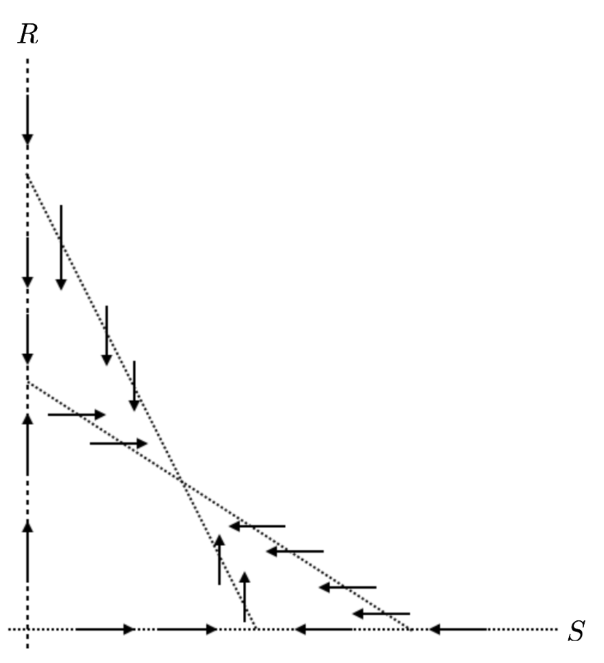
A certain system of differential equations for the variables \(R\) and \(S\) describes the interaction of rabbits and sheep grazing in the same field. On the phase plane below, dashed lines show the \(R\) and \(S\) nullclines along with their corresponding vectors.

Nullcline Plot

Question 4a:

Identify the \(R\) nullclines and explain how you know.

Solution to Question 4a:

Question 4b:

Identify the \(S\) nullclines and explain how you know.

Solution to Question 4b:

Question 4c:

Identify all equilibrium points.

Solution to Question 4c:

Question 4d:

Notice that the nullclines carve out 4 different regions of the first quadrant of the \(RS\) plane. In each of these 4 regions, add a prototypical-vector that represents the vectors in that region. That is, if you think the both \(R\) and \(S\) are increasing in a certain region then, draw a vector pointing up and to the right for that region.

Solution to Question 4d:

Question 4e:

What does this system seem to predict will happen to the rabbits and sheep in this field in the long run?

Solution to Question 4e:

Creative Commons License Information

Exploring Differential Equations by Adam Spiegler is licensed under a Creative Commons Attribution-NonCommercial-ShareAlike 4.0 International License.
Based on a work at https://github.com/CU-Denver-MathStats-OER/ODEs and original content created by Rasmussen, C., Keene, K. A., Dunmyre, J., & Fortune, N. (2018). Inquiry oriented differential equations: Course materials. Available at https://iode.sdsu.edu.

Plotting Phase Plane Portraits with phase_portrait

Loading ode_tools from GitHub

Importing the phase_portrait Plotting Function