import numpy as np
from scipy.integrate import odeint

# Definition of parameters
a = 3.  # rabbit growth/decay rate
b = -1.4  # rabbit interaction term with fox
c = -1.  # fox growth/decay rate
d = 0.8  # fox interaction term with rabbit

X0 = np.array([3, 2])  # initials conditions: 3 rabbits and 2 foxes

tspan = np.linspace(0, 15,  1000)  # time to evaluate solution

# Define differential equation
def dxdt(X, t, a,b,c,d):

    return np.array([
        a*X[0] + b*X[0]*X[1],
        c*X[1] + d*X[0]*X[1]
    ])

# Find solution
X = odeint(dxdt, X0, t=tspan, args = (a,b,c,d)) # solve system3.1: Introduction to Systems of ODEs
![]()
Reading: Notes on Diffy Q’s Section 3.1
Interacting Populations
Most species live in interaction with other species. For example, perhaps one species preys on another species, like foxes and rabbits. Below is a system of differential equations intended to predict future populations of rabbits and foxes over time, where \(R\) is the population (in hundreds) of rabbits at any time \(t\) and \(F\) is the population of foxes (in tens) at any time \(t\) (in years).
\[\begin{align} \frac{dR}{dt} &= 3R-1.4RF\\ \frac{dF}{dt} &= -F+0.8RF \end{align}\]
Question 1:
In earlier work with the rate of change equation \(\dfrac{dP}{dt}=kP\) we assumed that there was only one species, that the resources were unlimited, and that the species reproduced continuously. Which, if any, of these assumptions is modified and how is this modification reflected in the above system of differential equations?
Solution to Question 1:
Question 2:
Interpret the meaning of each term in the rate of change equations (e.g., how do you interpret or make sense of the \(-1.4RF\) term) and what are the implications of this term on the future predicted populations? Similarly for \(3R\), \(-F\), and \(0.8RF\).
Solution to Question 2:
Question 3:
Scientists studying a rabbit-fox population estimate that the current number of rabbits is 100 (\(R=1\)) and that the number of foxes is 10 (\(F=1\)). Use two steps of Euler’s method with step size of \(\Delta t =0.5\) to get numerical estimates for the future number of rabbits and foxes as predicted by the differential equations. Enter your answers in the table below.
Solution to Question 3:
| \(t\) (in years) | \(R\) (in hundreds) | \(F\) (in tens) | \(\dfrac{dR}{dt}\) | \(\Delta R\) | \(\dfrac{dF}{dt}\) | \(\Delta F\) |
|---|---|---|---|---|---|---|
| 0 | 1 | 1 | ?? | ?? | ?? | ?? |
| 0.5 | ?? | ?? | ?? | ?? | ?? | ?? |
| 1 | ?? | ?? | ?? | ?? | ?? | ?? |
Visualizing Solutions to a System of Differential Equations
We will continue working with the rabbit and fox population model below:
\[\begin{align} \frac{dR}{dt} &= 3R-1.4RF\\ \frac{dF}{dt} &= -F+0.8RF \end{align}.\]
If initially there are \(R=3\) (300 rabbits) and \(F=2\) (20 foxes), then the solution can be plotted in 3-dimensions as shown below.
- Run the first code cell (without any edits). The first code cell defines the parameters of the model and the initial values.
- Then run the second code cell (without any edits) to plot the solution in \(\mathbb{R}^3\).
import matplotlib.pyplot as plt

plt.figure(figsize=(8, 8))
ax = plt.axes(projection='3d')

ax.plot3D(tspan, X[:,0], X[:,1])
ax.set_xlabel('Time')
ax.set_ylabel('Rabbits')
ax.set_zlabel('Foxes')

plt.tight_layout()
2-Dimensional Projections
In our interacting rabbit and fox model, we have three variables \(R\), \(F\), and \(t\). From the solution in the \(3\)-dimensional plot above, we can better understand the dynamics of these two interacting species.
- How does the rabbit population change with time?
- How does the fox population change with time?
- How do the rabbit and fox populations interact with each over time?
A useful tool in mathematics for interpreting the relation between three variables is to consider pairwise relations. Graphically, this is equivalent to projecting the curve in 3 dimensional space above onto different 2 dimensional planes.
Question 4:
We would like to make future predictions for our rabbit-fox system
\[\begin{align} \frac{dR}{dt} &= 3R-1.4RF \\ \frac{dF}{dt} &= -F+0.8RF \end{align}\]
if at time \(t=0\) we initially have 300 rabbits (\(R=3\)) and 20 foxes (\(F=2\)).
Question 4a: Rabbits and Time
Run the code cell below to plot the graph of \(R\) vs \(t\).
- Use the graph to describe how the rabbit population will change as time goes on.
- Based on the graph, what type of function(s) would you use to model the solution \(R=f(t)\)? Explain how you determined your answer.
Solution to Question 4a:
Write your interpretation in the space below.
fig = plt.figure(figsize=(12,6))

ax1 = fig.add_subplot(1, 2, 1, projection='3d')
ax1.plot(tspan, X[:,0], 'r:', zdir='z', zs=0, alpha=.8)
ax1.plot3D(tspan, X[:,0], X[:,1])
ax1.set_xlabel('Time')

ax2 = fig.add_subplot(1, 2, 2)
ax2.plot(tspan, X[:,0], 'r-', alpha=.5)
ax2.grid()
ax2.set_xlabel('Time')
ax2.set_ylabel('Rabbits')
plt.tight_layout()
Question 4b: Foxes and Time
Run the code cell below to plot the graph of \(F\) vs \(t\).
- Use the graph to describe how the fox population will change as time goes on.
- Based on the graph, what type of function(s) would you use to model the solution \(F=g(t)\)? Explain how you determined your answer.
Solution to Question 4b:
Write your interpretation in the space below.
fig = plt.figure(figsize=(12,6))
ax1 = fig.add_subplot(1, 2, 1, projection='3d')
ax1.plot(tspan, X[:,1], 'g:', zdir='y', zs=40, alpha=.8)
ax1.plot3D(tspan, X[:,0], X[:,1])
ax1.set_xlabel('Time')

ax2 = fig.add_subplot(1, 2, 2)

ax2.plot(tspan, X[:,1], 'g-')
ax2.grid()
ax2.set_xlabel('Time')
ax2.set_ylabel('Foxes')
plt.tight_layout()
Question 4c: Rabbits and Foxes
Run the code cell below to plot the graph of \(R\) vs \(F\). Then use the graph to describe how the rabbit and fox populations interact with each other over time.
Solution to Question 4c:
Write your interpretation in the space below.
fig = plt.figure(figsize=(12,6))
ax1 = fig.add_subplot(1, 2, 1, projection='3d')

ax1.plot(X[:,0], X[:,1], 'k:', zdir='x', zs=0, alpha=.5)
ax1.plot3D(tspan, X[:,0], X[:,1])
ax1.set_xlabel('Time')

ax2 = fig.add_subplot(1, 2, 2)

ax2.plot(X[:,0], X[:,1], 'k-', alpha=.5)
ax2.grid()
ax2.set_xlabel('Rabbits')
ax2.set_ylabel('Foxes')
plt.tight_layout()
Question 5:
Suppose the current number of rabbits is \(R=3\) (300 rabbits) and the number of foxes is \(F=0\). Without using any technology and without making any calculations, what does the system of rate of change equations (same one as Question 4) predict for the future number of rabbits and foxes? Explain your reasoning.
Solution to Question 5:
Question 6:
Now use the code cells in parts (a)-(c) below to check your answer in Question 5 (with initial population \(R=3\) and \(F=0\)).
Question 6a: Plotting Rabbits vs Time
Run the code cell below to check your answer.
#import numpy as np
#from scipy.integrate import odeint

# Definition of parameters
#a = 3.  # rabbit growth/decay rate
#b = -1.4  # rabbit interaction term with fox
#c = -1.  # fox growth/decay rate
#d = 0.8  # fox interaction term with rabbit

X0 = np.array([3, 0])  # initials conditions: 3 rabbits and 0 foxes

tspan = np.linspace(0, 15,  1000)  # time to evaluate solution

# Define differential equation
def dxdt(X, t, a,b,c,d):

    return np.array([
        a*X[0] + b*X[0]*X[1],
        c*X[1] + d*X[0]*X[1]
    ])

# Find solution
X = odeint(dxdt, X0, t=tspan, args = (a,b,c,d)) # solve system

# Plot solution
fig = plt.figure(figsize=(12,6))

ax1 = fig.add_subplot(1, 2, 1, projection='3d')
ax1.plot(tspan, X[:,0], 'r:', zdir='z', zs=0, alpha=.8)
ax1.plot3D(tspan, X[:,0], X[:,1])
ax1.set_xlabel('Time')

ax2 = fig.add_subplot(1, 2, 2)
ax2.plot(tspan, X[:,0], 'r-', alpha=.5)
ax2.grid()
ax2.set_xlabel('Time')
ax2.set_ylabel('Rabbits')
plt.tight_layout()
Question 6b: Plotting Foxes vs Time
Run the code cell below to check your answer.
fig = plt.figure(figsize=(12,6))
ax1 = fig.add_subplot(1, 2, 1, projection='3d')
ax1.plot(tspan, X[:,1], 'g:', zdir='y', zs=40, alpha=.8)
ax1.plot3D(tspan, X[:,0], X[:,1])
ax1.set_xlabel('Time')

ax2 = fig.add_subplot(1, 2, 2)

ax2.plot(tspan, X[:,1], 'g-')
ax2.grid()
ax2.set_xlabel('Time')
ax2.set_ylabel('Foxes')
plt.tight_layout()
Question 6c: Plotting Rabbits vs Foxes
Run the code cell below to check your answer.
fig = plt.figure(figsize=(12,6))
ax1 = fig.add_subplot(1, 2, 1, projection='3d')

ax1.plot(X[:,0], X[:,1], 'm:', zdir='x', zs=0, alpha=.5)
ax1.plot3D(tspan, X[:,0], X[:,1])
ax1.set_xlabel('Time')

ax2 = fig.add_subplot(1, 2, 2)

ax2.plot(X[:,0], X[:,1], 'm-', alpha=.5)
ax2.grid()
ax2.set_xlabel('Rabbits')
ax2.set_ylabel('Foxes')
plt.tight_layout()
Question 7:
Using initial condition \(R = 3\) (300 rabbits) and \(F = 0\) (no foxes), tell the story (in words) of what happens to the rabbit and fox population as time continues.
Solution to Question 7:
Question 8:
What would it mean for the rabbit-fox system to be in equilibrium? Are there any equilibrium solutions to this system of rate of change equations? If so, determine all equilibrium solutions and generate the 3D and other views for each equilibrium solution.
Solution to Question 8:
Question 9:
For single differential equations, we classified equilibrium solutions as stable (attractors), unstable repellers, or semi-stable (nodes). For each of the equilibrium solutions in the previous question, create your own terms to classify the equilibrium solutions in and briefly explain your reasons behind your choice of terms.
Solution to Question 9:
The Phase Plane: Visualizing Solutions to Systems
One view of solutions for studying solutions to systems of autonomous (independent of \(t\)) differential equations of the form
\[\begin{aligned} \frac{dx}{dt} &= f(x,y)\\ \frac{dy}{dt} &= g(x,y) \end{aligned}\]
is in the \(xy\)-plane, called the phase plane.
- The phase plane is the analog to the phase line for a single autonomous differential equation.
- In the Rabbit-Fox example, these are the plots of \(F\) vs \(R\).
Question 10:
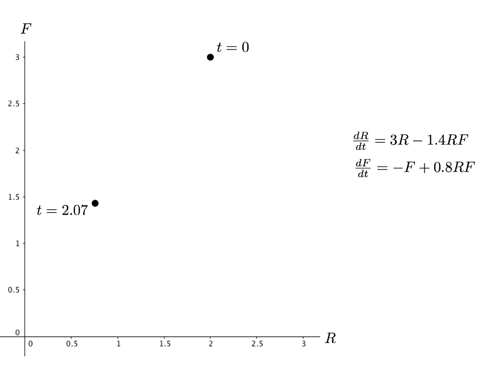
Consider the rabbit-fox system of differential equations
\[\begin{align} \frac{dR}{dt} &= 3R-1.4RF \\ \frac{dF}{dt} &= -F+0.8RF \end{align}\]
and the graph of the solution with initial condition \((2,3)\), as viewed in the phase plane (that is, the \(RF\)-plane). The two points in the table below are on the same solution curve. Recall that the solutions we’ve seen in the past are closed curves, but the solution could be moving clockwise or counterclockwise. Fill in the following table and decide which way the solution is moving, and explain your reasoning.
Solution to Question 10:
| \(t\) (in years) | \(R\) (in hundreds) | \(F\) (in tens) | \(\dfrac{dR}{dt}\) | \(\dfrac{dF}{dt}\) | \(\dfrac{dF}{dR}\) |
|---|---|---|---|---|---|
| \(0\) | \(2\) | \(3\) | Fill in your answer here | Fill in your answer here | Fill in your answer here |
| \(2.07\) | \(0.756\) | \(1.431\) | Fill in your answer here | Fill in your answer here | Fill in your answer here |
Comment on which direction (clockwise or counterclockwise) the solution rotates around the curve.
Question 11:
Consider plotting additional vectors in phase plane from Question 10 for the system
\[\begin{align} \frac{dR}{dt} &= 3R-1.4RF \\ \frac{dF}{dt} &= -F+0.8RF \end{align}\]
at the points \((R,F)\) in the table below. Fill in the blanks below and comment on whether you notice anything interesting about these vectors.
| \(R\) | \(F\) | \(\dfrac{dR}{dt}\) | \(\dfrac{dF}{dt}\) | \(\dfrac{dF}{dR}\) |
|---|---|---|---|---|
| \(1.25\) | \(0\) | ?? | ?? | ?? |
| \(1.25\) | \(1\) | ?? | ?? | ?? |
| \(1.25\) | \(2\) | ?? | ?? | ?? |
| \(1.25\) | \(3\) | ?? | ?? | ?? |
Solution to Question 11:
Replace each ?? with an appropriate value. Then comment on anything interesting you observe.
Creative Commons License Information

Exploring Differential Equations by Adam Spiegler is licensed under a Creative Commons Attribution-NonCommercial-ShareAlike 4.0 International License.
Based on a work at https://github.com/CU-Denver-MathStats-OER/ODEs and original content created by Rasmussen, C., Keene, K. A., Dunmyre, J., & Fortune, N. (2018). Inquiry oriented differential equations: Course materials. Available at https://iode.sdsu.edu.