# loads dplyr package
library(dplyr)1.2: Exploring Categorical Data
Click ![]() to open an interactive version of the full text section.
to open an interactive version of the full text section.
Additional Reading:
- See Overview of Plotting Data in R for further reading and examples about plotting in R.
- See Fundamentals of Working with Data for more information about data types and structures in R.
- The R Graph Gallery has examples of many other types of graphs.
An Overview of Exploratory Data Analysis
Exploratory data analysis, or EDA for short, can be thought of as a cycle:
- Generate questions about our data.
- Search for answers by visualizing, transforming, and modeling our data.
- Use what we learn to refine your questions and/or generate new questions.
The main goal of EDA is to develop an understanding of your data. When we ask a question, the question focuses our attention on a specific part of the data set and helps us decide which graphs, models, or transformations to make.
Loading the dplyr Package
The dplyr package is perhaps one of the most useful R packages for data wrangling and EDA. Data wrangling is generally the cleaning, reorganizing, and transforming data so it can be more easily analyzed. dplyr also contains data sets that we can use to practice our wrangling and visualization skills. In this lab, we will work with the data set called storms.
- See official dplyr documentation for a comprehensive tutorial.
- Run the code cell below to load the
dplyrpackage.
Finding Help Documentation
- The code cell below opens a glossary tab of all (most?) functions and data in the package
dplyr.
# open glossary of dplyr functions
help(package = "dplyr")- The code cell below opens a help tab with information about the
stormsdata set.
# opens help tab with info about storms data set
?storms
The Structure of Data
Data frames are two-dimensional data objects and are the fundamental data structure used by most of R’s libraries of functions and data sets.
- Tabular data is tidy if each row corresponds to a different observation and each column corresponds to a different variable.
Each column of a data frame is a variable (stored as a vector) of possibly different data types.
- If a variable is measured or counted by a number, it is called a quantitative or numerical variable.
- Quantitative variables may be discrete (integers) or continuous (decimals).
- If a variable groups observations into different categories or rankings, it is a qualitative or categorical variable.
- The different categories of a qualitative variable are called levels or classes.
- Levels are typically labeled with descriptive character strings or integers.
- Levels may or may not have an ordering.
- An ordinal variable is when the levels of a categorical variable do have a specified order.
- The different categories of a qualitative variable are called levels or classes.
Exploring Our Data
Below are some common functions used to get a first introduction to our data:
summary(df)gives numerical summary of all variables in data frame with generic namedf.glimpse(df)gives a glimpse of the data framedf.str(df)summarizes the structure of all variables in data framedfhead(df)view first 6 rows in data frame.tail(df)view last 6 rows in data frame.View(df)to view the full data frame.- It typically is not recommended to include a
View()command in your work since that opens the entire data set. - The goal of EDA is to provide nice summaries of a data set so we do not need to look at all the raw data!
Question 1
Let’s get to know the storms data set. Using some (or all) of the commands above, answer the following questions:
- How many observations are in data set
storms? - How many variables are
storms?- Which variables are quantitative and which are categorical?
- Which categorical variables have a ranking? Which do not?
- Hint: Avoid using the
View()function. Instead, usehead()ortail()if you want to get a sense of what the raw data looks like.
Experiment with some of the functions in the code cell below to answer the questions. Then type your answer in the space below.
summary(storms) # summary of each variable in storms name year month day
Length:19537 Min. :1975 Min. : 1.000 Min. : 1.00
Class :character 1st Qu.:1994 1st Qu.: 8.000 1st Qu.: 8.00
Mode :character Median :2004 Median : 9.000 Median :16.00
Mean :2003 Mean : 8.706 Mean :15.73
3rd Qu.:2013 3rd Qu.: 9.000 3rd Qu.:24.00
Max. :2022 Max. :12.000 Max. :31.00
hour lat long status
Min. : 0.000 Min. : 7.00 Min. :-136.90 tropical storm :6830
1st Qu.: 5.000 1st Qu.:18.30 1st Qu.: -78.80 hurricane :4803
Median :12.000 Median :26.60 Median : -62.30 tropical depression:3569
Mean : 9.101 Mean :27.01 Mean : -61.56 extratropical :2151
3rd Qu.:18.000 3rd Qu.:33.80 3rd Qu.: -45.50 other low :1453
Max. :23.000 Max. :70.70 Max. : 13.50 subtropical storm : 298
(Other) : 433
category wind pressure tropicalstorm_force_diameter
Min. :1.000 Min. : 10.00 Min. : 882.0 Min. : 0.0
1st Qu.:1.000 1st Qu.: 30.00 1st Qu.: 986.0 1st Qu.: 0.0
Median :1.000 Median : 45.00 Median :1000.0 Median : 110.0
Mean :1.896 Mean : 50.05 Mean : 993.5 Mean : 147.9
3rd Qu.:3.000 3rd Qu.: 65.00 3rd Qu.:1007.0 3rd Qu.: 220.0
Max. :5.000 Max. :165.00 Max. :1024.0 Max. :1440.0
NA's :14734 NA's :9512
hurricane_force_diameter
Min. : 0.00
1st Qu.: 0.00
Median : 0.00
Mean : 14.92
3rd Qu.: 0.00
Max. :300.00
NA's :9512 #head(storms) # prints first 6 rows to screen
#tail(storms) # prints last 6 rows to screen
#glimpse(storms) # gives a glimpse of the data set
#str(storms) # summary of data structureSolution to Question 1
Question 2:
What additional information would you like to know about the storms data set that you were unable to find? What questions do you have about the data? In particular, what data is missing and why?
Solution to Question 2:
Data Types
R has 6 basic data types:
- character: collections of characters. E.g.,
"a","hello world!" - double: decimal numbers. e.g.,
1.2,1.0 - integer: whole numbers. In R, you must add
Lto the end of a number to specify it as an integer. E.g.,1Lis an integer but1is a double. - logical: Boolean values,
TRUEandFALSE - complex: complex numbers. E.g.,
1+3i - raw: a type to hold raw bytes.
See the Appendix for an Fundamentals of Working with Data for more information.
Checking Data Types Using typeof()
- The
typeof()function returns the R internal type or storage mode of any object.
typeof(1.0)[1] "double"typeof(2)[1] "double"typeof(3L)[1] "integer"typeof("hello")[1] "character"typeof(TRUE)[1] "logical"typeof(storms$status)[1] "integer"typeof(storms$year)[1] "double"typeof(storms$name)[1] "character"Extracting a Variable By Name with $
In the command typeof(storms$status), notice we refer to just the status variable of the storms data frame. A variable from a data frame may be extracted using $ and then specifying the name of the desired variable.
- First indicate the name of the data frame,
storms. - Followed by a dollar sign
$. - Then indicate the name of the variable, for example
wind. - The
storms$windis a vector that contains the wind speed of each storm.
is.vector(storms) # storms is not a vector[1] FALSEis.data.frame(storms) # storms is a data frame[1] TRUEis.data.frame(storms$wind) # status is not a data frame[1] FALSEis.vector(storms$wind) # status is a vector[1] TRUEInvestigating Data Types with is.numeric()
- The
is.numeric(x)function tests whether or not an objectxis numeric. - The
is.character(x)function tests whetherxis a character or not. - The
is.factor(x)function tests whetherxis a factor or not. - Note: Categorical data is typically stored as a
factorin R.
is.numeric(storms$year) # year is numeric[1] TRUEis.numeric(storms$category) # category is also numeric[1] TRUEis.numeric(storms$name) # name is not numeric[1] FALSEis.character(storms$name) # name is character string[1] TRUEis.numeric(storms$status) # status is not numeric[1] FALSEis.character(storms$status) # status is not a character[1] FALSEis.factor(storms$status) # status is a factor which is categorical[1] TRUEConverting Decimals to Integers
From the summary of the storms data set we first found above, we see that the variables year and month are being stored as double. These variables actually are integer values.
We can convert another variable of one format into another format using as.[new_datatype]()
- For example, to convert to year to
integer, we useas.integer(storms$year). - To convert a data type to character, we can use
as.character(x). - To convert to a decimal (
double), we can useas.numeric(x)
typeof(storms$year)[1] "double"typeof(storms$month)[1] "double"storms$year <- as.integer(storms$year)
storms$month <- as.integer(storms$month)
typeof(storms$year)[1] "integer"typeof(storms$month)[1] "integer"Converting to Categorical Data with factor()
Sometimes we think a variable is one data type, but it is actually being stored (and thus interpreted by R) as a different data type. One common issue is categorical data is stored as characters or integers. We would like observations with the same values to be group together.
- The
statusvariable instormsis being properly stored as afactor. - The
categoryvariable instormsis being stored as anumericsince the classes are integers.
summary(storms$category) Min. 1st Qu. Median Mean 3rd Qu. Max. NA's
1.000 1.000 1.000 1.896 3.000 5.000 14734 The summary of category computes statistics such as mean and median. Typically with categorical data, we prefer to count how many observations are in each class of the variable.
- In the code cell below, we convert
categoryto a factor, and then observe the resulting summary.
storms$category <- factor(storms$category)
summary(storms$category)
1 2 3 4 5 NA's
2548 993 593 553 116 14734 Assignment of New Objects
Notice in the code cell above, we replace the original integers in the category column with a integers that are now stored as different levels of a categorical variable.
- To store a data structure in the computer’s memory we must assign it a name.
- In this case, we choose to give the variable the same name, an therefore overwrite the original
categorycolumn.
- In this case, we choose to give the variable the same name, an therefore overwrite the original
- Data structures can be stored using the assignment operator
<-.
Frequency and Relative Frequency Tables
table(x)creates a frequency table for categorical variablex.table(x, y)creates a two-way (or contingency) table for two categorical variablesxandyprop.table([table])creates a relative frequency table relative to the grand total.- The input of
prop.table()must be a table. prop.table([table], 1)creates a relative frequency table relative to total in each row.prop.table([table], 2)creates a relative frequency table relative to total in each column.
- The input of
Question 3
Which month over the period from 1975-2021 had the greatest number of subtropical storms? Which table did you use to help answer your question?
Which month over the period from 1975-2021 had the greatest proportion of subtropical storms? Which table did you use to help answer your question?
Run each of the four code cells below, and after interpreting the output of each, answer the questions in the space below.
my.table <- table(storms$month, storms$status)  # gives counts
my.table
     disturbance extratropical hurricane other low subtropical depression
  1            0            29         5         5                      0
  4            0            40         0         0                      4
  5            0            18         0        49                      5
  6           35           130        18        84                     35
  7           46           135       221       181                     11
  8           25           275      1038       319                     36
  9           41           800      2464       473                     34
  10          16           527       803       226                     22
  11           8           183       221        85                      4
  12           0            14        33        31                      0

     subtropical storm tropical depression tropical storm tropical wave
  1                  6                   2             23             0
  4                  3                   1             18             0
  5                 20                  49             60             0
  6                 12                 213            282             0
  7                  6                 399            645             7
  8                 23                 975           1696            55
  9                 72                1331           2522            41
  10                66                 429           1049             0
  11                48                 149            464             8
  12                42                  21             71             0
prop.grand <- prop.table(my.table) # gives proportions relative to grand total
round(prop.grand, 4)
     disturbance extratropical hurricane other low subtropical depression
  1       0.0000        0.0015    0.0003    0.0003                 0.0000
  4       0.0000        0.0020    0.0000    0.0000                 0.0002
  5       0.0000        0.0009    0.0000    0.0025                 0.0003
  6       0.0018        0.0067    0.0009    0.0043                 0.0018
  7       0.0024        0.0069    0.0113    0.0093                 0.0006
  8       0.0013        0.0141    0.0531    0.0163                 0.0018
  9       0.0021        0.0409    0.1261    0.0242                 0.0017
  10      0.0008        0.0270    0.0411    0.0116                 0.0011
  11      0.0004        0.0094    0.0113    0.0044                 0.0002
  12      0.0000        0.0007    0.0017    0.0016                 0.0000

     subtropical storm tropical depression tropical storm tropical wave
  1             0.0003              0.0001         0.0012        0.0000
  4             0.0002              0.0001         0.0009        0.0000
  5             0.0010              0.0025         0.0031        0.0000
  6             0.0006              0.0109         0.0144        0.0000
  7             0.0003              0.0204         0.0330        0.0004
  8             0.0012              0.0499         0.0868        0.0028
  9             0.0037              0.0681         0.1291        0.0021
  10            0.0034              0.0220         0.0537        0.0000
  11            0.0025              0.0076         0.0237        0.0004
  12            0.0021              0.0011         0.0036        0.0000
prop.row <- prop.table(my.table, 1) # gives proportions relative to row totals
round(prop.row, 4)
     disturbance extratropical hurricane other low subtropical depression
  1       0.0000        0.4143    0.0714    0.0714                 0.0000
  4       0.0000        0.6061    0.0000    0.0000                 0.0606
  5       0.0000        0.0896    0.0000    0.2438                 0.0249
  6       0.0433        0.1607    0.0222    0.1038                 0.0433
  7       0.0279        0.0818    0.1339    0.1096                 0.0067
  8       0.0056        0.0619    0.2337    0.0718                 0.0081
  9       0.0053        0.1029    0.3168    0.0608                 0.0044
  10      0.0051        0.1679    0.2559    0.0720                 0.0070
  11      0.0068        0.1564    0.1889    0.0726                 0.0034
  12      0.0000        0.0660    0.1557    0.1462                 0.0000

     subtropical storm tropical depression tropical storm tropical wave
  1             0.0857              0.0286         0.3286        0.0000
  4             0.0455              0.0152         0.2727        0.0000
  5             0.0995              0.2438         0.2985        0.0000
  6             0.0148              0.2633         0.3486        0.0000
  7             0.0036              0.2417         0.3907        0.0042
  8             0.0052              0.2195         0.3818        0.0124
  9             0.0093              0.1711         0.3242        0.0053
  10            0.0210              0.1367         0.3343        0.0000
  11            0.0410              0.1274         0.3966        0.0068
  12            0.1981              0.0991         0.3349        0.0000
prop.col <- prop.table(my.table, 2) # gives proportions relative to column totals
round(prop.col, 4)
     disturbance extratropical hurricane other low subtropical depression
  1       0.0000        0.0135    0.0010    0.0034                 0.0000
  4       0.0000        0.0186    0.0000    0.0000                 0.0265
  5       0.0000        0.0084    0.0000    0.0337                 0.0331
  6       0.2047        0.0604    0.0037    0.0578                 0.2318
  7       0.2690        0.0628    0.0460    0.1246                 0.0728
  8       0.1462        0.1278    0.2161    0.2195                 0.2384
  9       0.2398        0.3719    0.5130    0.3255                 0.2252
  10      0.0936        0.2450    0.1672    0.1555                 0.1457
  11      0.0468        0.0851    0.0460    0.0585                 0.0265
  12      0.0000        0.0065    0.0069    0.0213                 0.0000

     subtropical storm tropical depression tropical storm tropical wave
  1             0.0201              0.0006         0.0034        0.0000
  4             0.0101              0.0003         0.0026        0.0000
  5             0.0671              0.0137         0.0088        0.0000
  6             0.0403              0.0597         0.0413        0.0000
  7             0.0201              0.1118         0.0944        0.0631
  8             0.0772              0.2732         0.2483        0.4955
  9             0.2416              0.3729         0.3693        0.3694
  10            0.2215              0.1202         0.1536        0.0000
  11            0.1611              0.0417         0.0679        0.0721
  12            0.1409              0.0059         0.0104        0.0000
Solution to Question 3
Visualizing Categorical Data
There are many different ways we can great visualizations to gain insight into our data and search for possible patterns and relations between different variables.
- For one categorical variable: Bar charts (or bar plots) and pie charts are commonly used.
- For two categorical variables: Grouped and stacked bar charts are commonly used.
Creating Bar Charts with plot()
- The
plot()function is the most broadly used function for plotting different data types. - The type of plot generated by
plot()depends on the data type(s) and the number of variable(s) we input.- If we input one categorical variable that is stored as
factor, we get a bar chart. - If we input one quantitative variable, the plot is typically not very useful.
- If a categorical variable is stored incorrectly as quantitative, we do not get an appropriate plot.
- If we input one categorical variable that is stored as
- If we use
plot()to display a categorical variable, the variable must be stored as a factor!- Recall we converted
categoryto afactorin a previous code cell. - The variable
monthis a quantitative variable.
- Recall we converted
# plots appear in an array with 1 row and 2 columns
par(mfrow = c(1, 2))  # create an array of plots

plot(storms$category,  # categorical data
     main = "Hurricanes by Category",  # main title
     xlab = "Hurricane Category",  # horizontal axis label
     ylab = "Frequency",  # vertical axis label
     col = "steelblue")  # fill color of bars)

plot(storms$month,  # quantitative data
     main = "Not Number of Storms in Month",  # main title
     xlab = "Index (Row of Observation)",  # horizontal axis label
     ylab = "Month")  # vertical axis label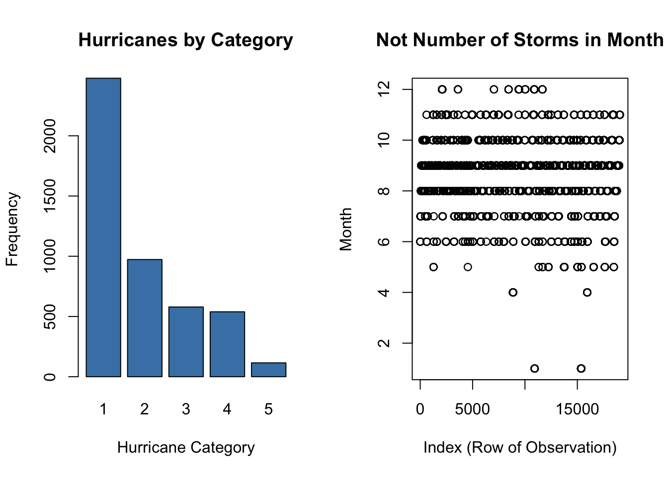
Creating Bar Charts and Pie Charts from a Table
If we want to keep month stored as an integer, but would like to create a visualization to display the number of storms that occurred in each month, we can:
- First use the
table()function to count how many storms occurred in each month. - Then create a bar chart using the
barplot()function or pie chart usingpie().
# plots appear in an array with 1 row and 2 columns
par(mfrow = c(1, 2))  # create an array of plots

month.table <- table(storms$month)  # create table of month counts
category.table <- table(storms$category)  # create table of category counts

barplot(month.table,  # input table of month counts
        main = "Storms in Each Month",  # main title
        xlab = "Month",  # horizontal axis label
        ylab = "Frequency",  # vertical axis label
        col = "seagreen")  # fill color of bars

pie(category.table,  # input table of category counts
    main = "Hurricanes by Category")  # main title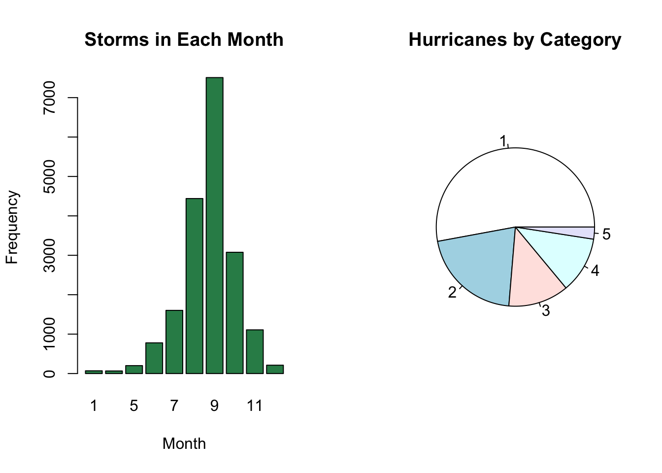
Note, pie() and barplot() both take tables as inputs. Even if a variable is stored as a factor, we need to store the counts in a table first.
- The
categoryvariable instormsis stored as a factor, but the code below still crashes.
# see what happens if input is not a table
pie(storms$category)
Relationship Between Two Categorical Variables
Imagine we would like to compare the number of different category hurricanes that occurred in each month. In this case, we would like to compare two qualitative variables, namely category and month.
Grouped Frequency Bar Charts
To create a bar chart displaying the number of category hurricanes that occurred in each month:
- First create a two-way table of counts.
- The second variable (
month) is displayed on horizontal axis. - We get a separate bar for each level of the first variable (
category).
- The second variable (
- Input the table into the
barplot()function.- Note the option
beside = TRUEgroups the bars for each month. - The default option
beside = FALSEstacks the bars.
- Note the option
# two-way table of counts of category in each month
cat.table <- table(storms$category, storms$month)  # gives counts
# create a vector of colors
my.colors <- c("green", "purple", "grey", "red", "blue")
# create side by side bar chart
barplot(cat.table, # use counts from contingency table
beside = TRUE, # groups side-by-side
main = "Category Hurricanes By Month", # main title
xlab = "Month", # horizontal axis label
col = my.colors, # fill color of bars
ylab = "Frequency") # vertical axis label
# add a legend to plot
legend(x="topleft", # place legend in top left
legend=rownames(cat.table), # get labels from row name in contingency table
fill = my.colors) # use same fill colors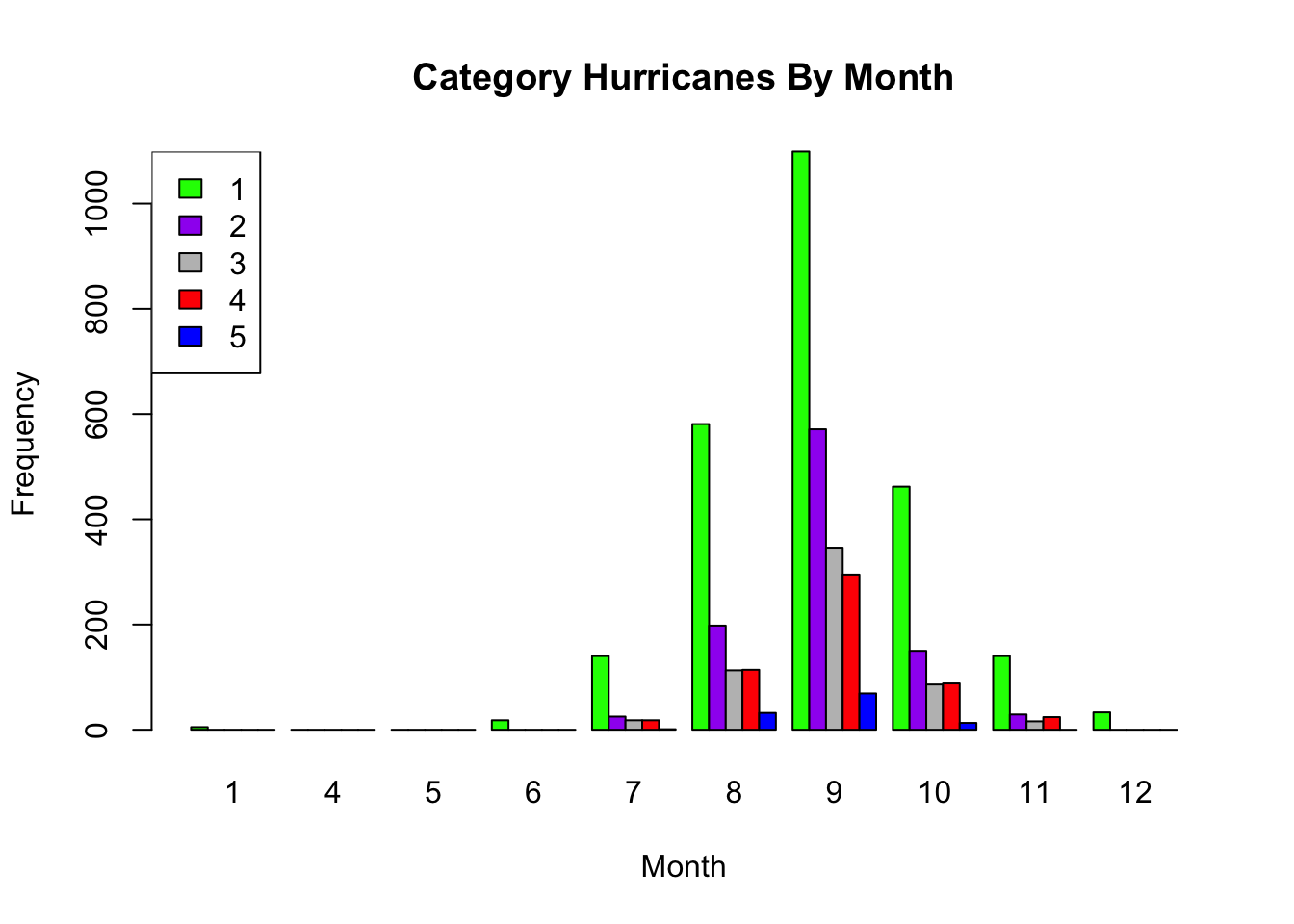
Stacked Relative Frequency Bar Charts
To create a bar chart displaying the relative frequency (or proportion) of category hurricanes that occurred in each month:
- First create a two-way table of relative frequencies.
- Pay attention to whether you want the proportions relative to grand, row, or column totals.
- Input the table into the
barplot()function.- The default option
beside = FALSEstacks the bars.
- The default option
cat.grand <- prop.table(cat.table)  # gives proportions relative to grand total
cat.row <- prop.table(cat.table, 1)  # gives proportions relative to row totals
cat.col <- prop.table(cat.table, 2) # gives proportions relative to column totalspar(mfrow = c(1, 3)) # create an array of plots
# create stacked bar chart 1
barplot(cat.grand, # use proportions from contingency table
main = "Category Hurricanes By Month", # main title
xlab = "Month", # horizontal axis label
col = my.colors, # color of bars
ylab = "Proportion") # vertical axis label
# add legend to plot
legend(x="topleft", # place legend in top left
legend=rownames(cat.grand), # get labels
fill = my.colors) # use same colors
##########
# create stacked bar chart 2
barplot(cat.row, # use proportions from contingency table
main = "Category Hurricanes By Month", # main title
xlab = "Month", # horizontal axis label
col = my.colors, # color of bars
ylab = "Proportion") # vertical axis label
# add legend to plot
legend(x="topleft", # place legend in top left
legend=rownames(cat.row), # get labels
fill = my.colors) # use same colors
###########
# create stacked bar chart 3
barplot(cat.col, # use proportions from contingency table
main = "Category Hurricanes By Month", # main title
xlab = "Month", # horizontal axis label
col = my.colors, # color of bars
ylab = "Proportion") # vertical axis label
# add legend to plot
legend(x="topleft", # place legend in top left
legend=rownames(cat.col), # get labels
fill = my.colors) # use same colors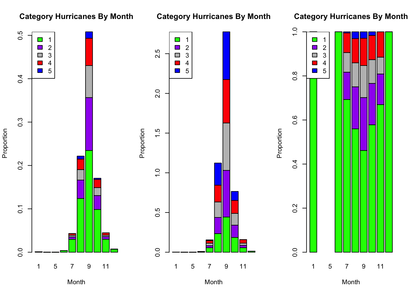
Note
A proportion greater than 1 in the middle bar chart means, for example, the sum of the all September proportions (one relative to each category total) adds up to \(2.8\) since in 4 out of the 5 possible hurricane categories September accounts for over half the total.
Question 4
Based on the three plots generated in the previous code cell, answer the questions below.
Which month has the most hurricanes?
In which month is the proportion of category 1 hurricanes greatest?
Solution to Question 4
Question 5
What are the the differences in the three plots in the output of the previous code cell? Which of the three bar plots above do you believe best visualizes the occurrence of different category hurricanes by month? Which plot do you think is the least useful overall? Explain why.
Solution to Question 5
Exploring the General Social Survey Data Set
The data set gss_cat can be accessed from the forcats package. Below is a quote taken from the website of the GSS Data Explorer website maintained by NORC at the University of Chicago
The General Social Survey (GSS) is a project of NORC at the University of Chicago, with principal funding from the National Science Foundation. Since 1972, the GSS has been monitoring societal change and studying the growing complexity of American society.
The GSS is a publicly available national resource, and is one of the most frequently analyzed sources of information in the social sciences. GSS Data Explorer is one of many ways that NORC supports the dissemination of GSS data for use by legislators, policymakers, researchers, educators and others.
# load the forcats package
library(forcats)
# open help documentation for gss_cat
?gss_cat# get numerical summary of variables
summary(gss_cat) year marital age race
Min. :2000 No answer : 17 Min. :18.00 Other : 1959
1st Qu.:2002 Never married: 5416 1st Qu.:33.00 Black : 3129
Median :2006 Separated : 743 Median :46.00 White :16395
Mean :2007 Divorced : 3383 Mean :47.18 Not applicable: 0
3rd Qu.:2010 Widowed : 1807 3rd Qu.:59.00
Max. :2014 Married :10117 Max. :89.00
NA's :76
rincome partyid relig
$25000 or more:7363 Independent :4119 Protestant:10846
Not applicable:7043 Not str democrat :3690 Catholic : 5124
$20000 - 24999:1283 Strong democrat :3490 None : 3523
$10000 - 14999:1168 Not str republican:3032 Christian : 689
$15000 - 19999:1048 Ind,near dem :2499 Jewish : 388
Refused : 975 Strong republican :2314 Other : 224
(Other) :2603 (Other) :2339 (Other) : 689
denom tvhours
Not applicable :10072 Min. : 0.000
Other : 2534 1st Qu.: 1.000
No denomination : 1683 Median : 2.000
Southern baptist: 1536 Mean : 2.981
Baptist-dk which: 1457 3rd Qu.: 4.000
United methodist: 1067 Max. :24.000
(Other) : 3134 NA's :10146 Question 6
Create a plot to visualize one categorical variable in the gss_cat data set. Based on your plot, comment on any interesting features of the variable you plotted.
# create a visualization for one categorical variableSolution to Question 6
Question 7
Create a plot to visualize the relationship between two categorical variables in the gss_cat data set. Based on your plot, comment on any interesting features or relations between two the variables you plotted.
# create a visualization to illustrate the relation
# between two categorical variables
Solution to Question 7

Statistical Methods: Exploring the Uncertain by Adam Spiegler is licensed under a Creative Commons Attribution-NonCommercial-ShareAlike 4.0 International License.