5.2: Bootstrap Confidence Intervals

In our work with bootstrap distributions, we explored how we can used data from one random sample picked from a population with unknown parameters to construct an approximation for a sampling distribution. From a bootstrap distribution, we can define a new estimator:

We defined the estimator $\hat{\theta}_{\rm{boot}}$ as the mean (expected) value of the bootstrap distribution.
We use the bootstrap standard error to estimate the variability or uncertainty in estimates due to the randomness of sampling.
We defined the bootstrap estimate of bias as $\mbox{Bias}_{\rm{boot}} \big( \hat{\theta}_{\rm{boot}} \big) = \hat{\theta}_{\rm{boot}} - \left( \mbox{observed sample statististic} \right)$.
- For example, in the case of estimating a population mean $\mu$, we have ${\color{dodgerblue}{\mbox{Bias}_{\rm{boot}} \big( \hat{\mu}_{\rm{boot}} \big) = \hat{\mu}_{\rm{boot}} - \bar{x}}}$.

In this section we will discuss how we can use the bootstrap standard error to account for the uncertainty in our estimate and to incorporate that uncertainty in our final estimate.

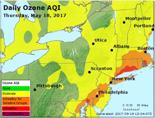
Case Study: Ozone Concentration in New York City

Map of Air Quality in Northeastern US — Credit: Northeast States for Coordinated Air Use Management (NESCAUM)

Accoording to the Unites States Environmental Protection Agency (EPA)¹:

Ozone (O3) is a highly reactive gas composed of three oxygen atoms. It is both a natural and a man-made product that occurs in the Earth’s upper atmosphere (the stratosphere) and lower atmosphere (the troposphere). Depending on where it is in the atmosphere, ozone affects life on Earth in either good or bad ways.

When the ozone concentration is greater, respiratory illnesses such as asthma, pneumonia, and bronchitis can become exacerbated. While the effects of short-term exposure to high ozone concentration are reversible, long-term exposure may not be reversible. The EPA sets Ozone National Ambient Air Quality Standards (NAAQS)². “The existing primary and secondary standards, established in 2015, are 0.070 parts per million (ppm)”, or equivalently 70 parts per billion (pbb).

We will begin todays work with bootstrap distributions investigating the following question:

Is the population of New York City experiencing long-term exposure to unhealthy levels of ozone?

Loading NYC Ozone Data

It is very likely you do not have the package lattice installed. You will need to first install the lattice package.

Go to the R Console window.
Run the command > install.packages("lattice").

You will only need to run the install.package() command one time. You can now access lattice anytime you like! However, you will need to run the command library(lattice) during any R session in which you want to access data from the lattice package. Be sure you have first installed the lattice package before executing the code cell below.

# be sure you have already installed the lattice package
library(lattice)  # loading permute package

Summarizing and Storing the Data

In the code cell below we summarize a data frame³ named environmental from the lattice package and store the ozone concentration data environmental$ozone to a vector named nyc.oz.

summary(environmental)  # numerical summary of each variable

     ozone         radiation      temperature         wind       
 Min.   :  1.0   Min.   :  7.0   Min.   :57.00   Min.   : 2.300  
 1st Qu.: 18.0   1st Qu.:113.5   1st Qu.:71.00   1st Qu.: 7.400  
 Median : 31.0   Median :207.0   Median :79.00   Median : 9.700  
 Mean   : 42.1   Mean   :184.8   Mean   :77.79   Mean   : 9.939  
 3rd Qu.: 62.0   3rd Qu.:255.5   3rd Qu.:84.50   3rd Qu.:11.500  
 Max.   :168.0   Max.   :334.0   Max.   :97.00   Max.   :20.700

nyc.oz <- environmental$ozone  # store ozone data to a vector

Question 1

We will use the sample data stored in nyc.oz to construct a bootstrap distribution that we can use to make predictions about the population of all times in New York City. Answer the questions below to get acquainted with the sample data.

Question 1a

How many observations are in the sample stored in nyc.oz? Describe the shape of the data in nyc.oz.

Solution to Question 1a

Question 1b

Based on the sample data in nyc.oz, give an estimate for the mean ozone concentration in New York City (over all days and times).

Solution to Question 1b

Bootstrap Distribution for a Proportion

The sample mean for ozone concentration is below the 70 ppb limit. However, from the plot in Question 1a, we see there are number of observations in the sample with an ozone concentration over 70 ppb.

sum(nyc.oz > 70)

[1] 24

What proportion of time in NYC is the ozone concentration greater than 70 ppb?

The sample proportion of observations with an ozone concentration greater than 70 pbb is $24/111 \approx 0.2162$. We calculate the sample proportion in two different ways below. In both methods, we use the logical test nyc.oz > 70 to help count the number of observations greater than 70 pbb.

Using a logical test in a sum() command and dividing by the sample size n.
Using a logical test in a mean() command sums and divides by $n$ at once.

# method 1
n <- length(nyc.oz)  # number of observations in sample
sum(nyc.oz > 70) / n  # sample proportion over 70 ppb

[1] 0.2162162

# method 2
mean(nyc.oz > 70)  # sample proportion over 70 ppb

[1] 0.2162162

Both methods are equivalent and we see that

\[\hat{p} = 0.2162 = 21.62 \%.\] Thus use the plug-in principle, a reasonable estimate for the proportion of all time that the ozone concentration in NYC is over 70 ppb (we denote the population proportion $p$) is

\[ p \approx \hat{p} = 0.2612.\] How certain can we be in this estimate? If we pick another sample of observations, would we get a similar estimate for $p$, or should we expect a lot of variability?

Question 2

Answer each part below to construct a bootstrap distribution for the sample proportion. Then use the result to answer the questions that follow.

Question 2a

Complete the code cell below to construct a bootstrap distribution for the sample proportion of observations with ozone concentration greater than 70 ppb.

Tip

There are two operations to complete inside the for loop:

Pick a bootstrap resample from the observed sample nyc.oz.
Calculate the proportion of observations in the bootstrap resample with ozone concentration greater than 70 ppb.

Solution to Question 2a

Replace all six ?? in the code cell below with appropriate code. Then run the completed code to generate a bootstrap distribution and mark the observed sample proportion (in red) and the mean of the bootstrap distribution (in blue) with vertical lines.

N <- 10^5  # Number of bootstrap samples
boot.prop <- numeric(N)  # create vector to store bootstrap proportions

# for loop that creates bootstrap dist
for (i in 1:N)
{
  x <- sample(??, size = ??, replace = ??)  # pick a bootstrap resample
  boot.prop[i] <- ??  # compute bootstrap sample proportion
}

# plot bootstrap distribution
hist(boot.prop,  
     breaks=20, 
     xlab = "p-hat, sample proportion",
     main = "Bootstrap Distribution for Sample Proportion")

# red line at the observed sample proportion
abline(v = ??, col = "firebrick2", lwd = 2, lty = 1)

# blue line at the center of bootstrap dist
abline(v = ??, col = "blue", lwd = 2, lty = 2)

Question 2b

Based on your answer to Question 2a, calculate bootstrap estimate for bias. Note answers will vary due to the randomness of bootstrapping in Question 2a.

Solution to Question 2b

# calculate bootstrap estimate of bias

Question 2c

Based on your answer to Question 2a, calculate the bootstrap estimate for the standard error of the sampling distribution for sample proportions. Note answers will vary due to the randomness of bootstrapping in Question 2a.

Solution to Question 2c

# calculate bootstrap standard error

Comparing Bootstrapping to CLT

Recall the Central Limit Theorem (CLT) for Proportions,

\[\widehat{P} \sim N \left( \mu_{\hat{P}}, \mbox{SE}(\widehat{P}) \right) = \left( {\color{tomato}{p}}, \sqrt{\frac{{\color{tomato}{p}}(1-{\color{tomato}{p}})}{n}} \right).\]

The population proportion $p$ is unknown, but we can use the plug-in principle and use the sample proportion ${\color{tomato}{\hat{p} = 0.2162}}$ in place to estimate the sampling distribution for the sample proportion:

\[\begin{aligned} \widehat{P} \sim N \left( \mu_{\hat{P}}, \mbox{SE}(\widehat{P}) \right) &= \left( {\color{tomato}{p}}, \sqrt{\frac{{\color{tomato}{p}}(1-{\color{tomato}{p}})}{n}} \right) \\ & \approx N\left( {\color{tomato}{0.2162}}, \sqrt{\frac{{\color{tomato}{0.2162}}(1-{\color{tomato}{0.2162}})}{111}} \right) \\ & \approx N( 0.2162, 0.0391). \end{aligned}\]

Method	Mean of Sampling Distribution	Standard Error
Bootstrap⁴	$0.2164$	$0.0390$
CLT with $\hat{p}$ in place of $p$	$0.2162$	$0.0391$

The two methods, bootstrap distribution and the estimate from using the CLT, give us consistent results!

Interval and Point Estimates

Usually when estimating an unknown population parameter, we give an interval estimate that gives range of plausible values for the parameter by accounting for the uncertainty due to the variability in sampling.

For example, using both mean and standard error from the bootstrap distribution in Question 2c, we could say

\[ p_{\rm over} \approx \hat{p}_{\rm boot} \color{dodgerblue}{\pm \mbox{SE}_{\rm boot} \left( \widehat{P} \right)} = 0.216 \color{dodgerblue}{\pm 0.039}.\]

An interval of plausible values for $p$ is from $0.177$ to $0.255$.
An estimate for a parameter with a single value is called a point estimate.
- Since there is variability from sample to sample, it is not very likely that our point estimate is perfectly accurate, but it is likely close.
- We get a very specific estimate that is very unlikely to equal the actual parameter value.
- This is like trying to catch a fish with a spear.
An estimate for a parameter with a range of values is called an interval estimate.
- By building some uncertainty into our estimate, we can be more confident the actual value of the parameter is somewhere inside the interval.
- However, our estimate is less specific.
- This is like trying to catch a fish with a net.
- We are more likely to catch fish even if we do not know specifically where the fish is!
We frequently estimate parameters with interval to account for the variability of sample statistics.

Man Throwing a Fishing Net — Credit: Rahil, Public Domain, Pixahive

Sealing Canoe Showing Method of Throwing Spear — Credit: Rahil, Public Domain, Pixahive

A 95% Bootstrap Percentile Confidence Interval

The interval between the $2.5$ and $97.5$ percentiles (or $0.025$ and $0.975$ quantiles) of the bootstrap distribution of a statistic is a 95% bootstrap percentile confidence interval for the corresponding parameter.

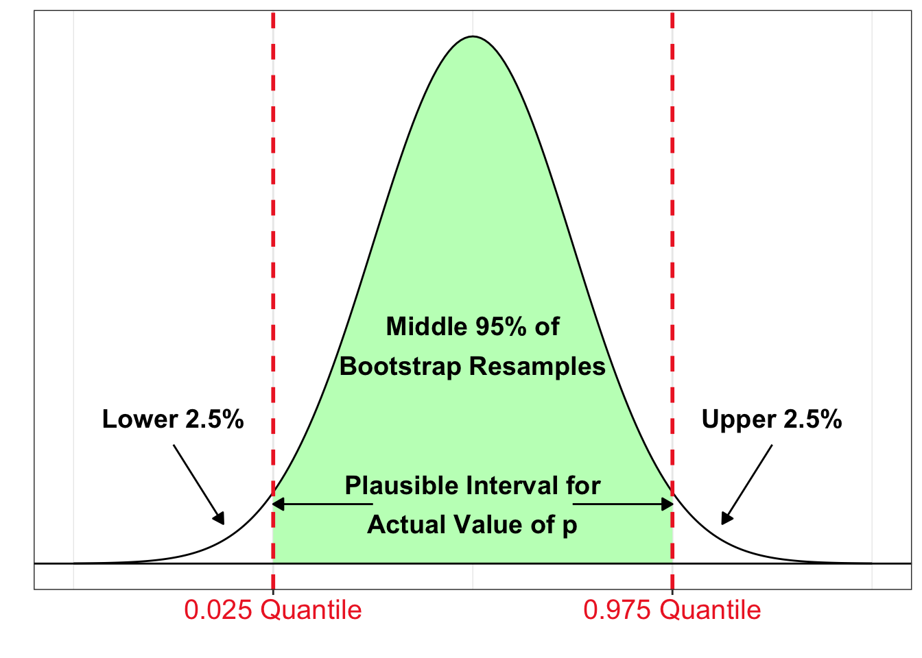
If most of the sample statistics are located in a certain interval of the bootstrap distribution, it seems plausible the true value of the parameter is in this interval!
We would say we are 95% confident that the interval contains the actual value of the population parameter since 95% of the bootstrap resamples are inside this interval.
In general, confidence interval estimates give a range of plausible values for the unknown value of the parameter.

Question 3

In Question 2, we created a bootstrap distribution (stored in the vector boot.prop) for the sample proportion of times the ozone concentration exceeds 70 ppb. One possible bootstrap distribution is plotted below. Bootstrap distributions will vary slightly depending on the 100,000 bootstrap resamples that are randomly selected.

# plot bootstrap distribution
hist(boot.prop,  
     breaks=20, 
     xlab = "p-hat, sample proportion",
     main = "Bootstrap Distribution for Sample Proportion")

# red line at the observed sample proportion
abline(v = mean(nyc.oz > 70), col = "firebrick2", lwd = 2, lty = 1)

# blue line at the center of bootstrap dist
abline(v = mean(boot.prop), col = "blue", lwd = 2, lty = 2)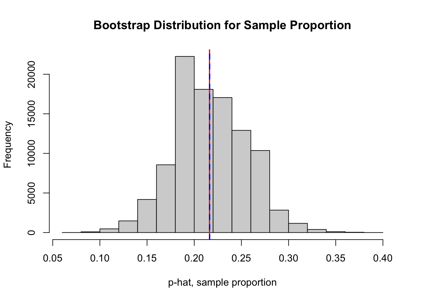

Question 3a

Using the bootstrap statistics stored in boot.prop, find the lower and upper cutoffs for a 95% bootstrap percentile confidence interval for the proportion of all times the ozone concentration in NYC exceeds 70 ppb.

Tip

Recall the quantile() function in R. Run the command ?quantile for a refresher!

Solution to Question 3a

Replace all four ?? in the code cell below with appropriate code. Then run the completed code to compute lower and upper cutoffs for a 95% bootstrap percentile confidence interval.

# find cutoffs for 95% bootstrap CI
lower.boot.95 <- quantile(??, probs = ??)  # find lower cutoff
upper.boot.95 <- quantile(??, probs = ??)  # find upper cutoff

# print values to screen
lower.boot.95
upper.boot.95

Based on the output above, a 95% bootstrap percentile confidence interval is from ?? to ??.

Question 3b

The code cell below plots a bootstrap distribution corresponding of the sample proportions stored in boot.prop along with two blue vertical lines to mark the lower and upper cutoffs for a 95% bootstrap percentile confidence interval. A red vertical line marks the value of the sample proportion we calculated from the original sample.

Run the code cell below to illustrate the confidence interval on the bootstrap distribution. There is nothing to edit in the code cell. Then in the space below, explain the practical meaning of the interval to a person with little to no background in statistics.

#################################
# code is ready to run!
# no need to edit the code cell
#################################

# plot bootstrap distribution
hist(boot.prop,  
     breaks=20, 
     xlab = "p-hat, sample proportion",
     main = "Bootstrap Distribution for Sample Proportion")

# red line at the observed sample proportion
abline(v = mean(nyc.oz > 70), col = "firebrick2", lwd = 2, lty = 1)

# blue lines marking cutoffs
abline(v = lower.boot.95, col = "blue", lwd = 2, lty = 2)
abline(v = upper.boot.95, col = "blue", lwd = 2, lty = 2)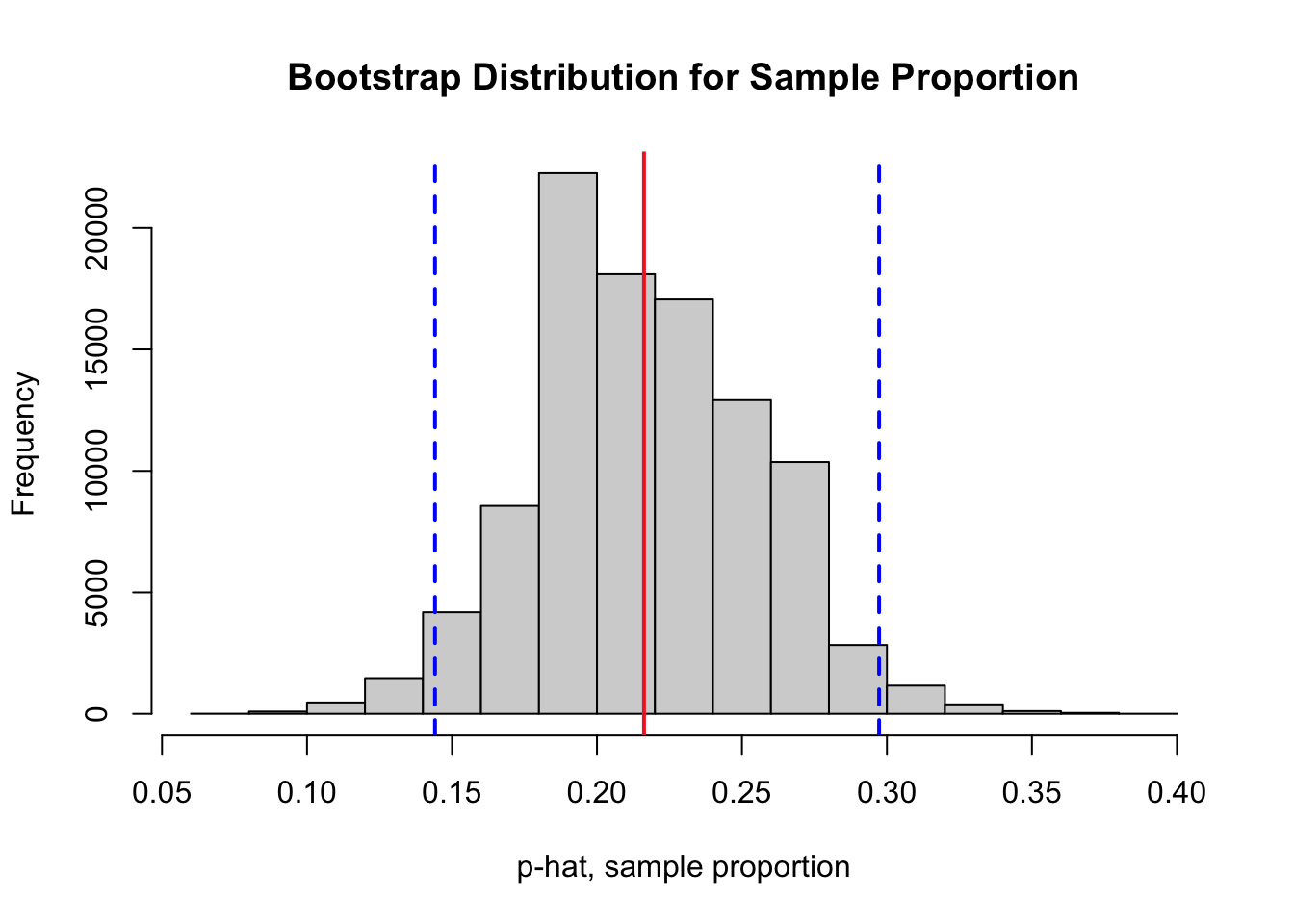

Solution to Question 3b

Interpret the confidence interval from Question 3a.

Question 3c

Sometimes, it is desirable to describe the interval as some value plus or minus some margin of error. Construct a symmetric 95% bootstrap confidence interval for the proportion of time the ozone concentration in NYC exceeds 70 ppb. Compare the symmetric confidence interval to your percentile confidence interval in Question 3a.

Tip

Recall for normal distributions, approximately 95% of the data is within 2 standard deviations of center of the distribution.

Solution to Question 3c

Replace each ?? in the code cell below with appropriate code.

?? - 2*??  # going 2 SE's below the observed sample proportion
?? + 2*??  # going 2 SE's above the observed sample proportion

Based on the output above, a symmetric 95% bootstrap confidence interval is from ?? to ??.

Adjusting the Confidence Level

We would expect the actual value of the unknown population parameter to equal the corresponding statistic calculated from one of the 100,000 bootstrap resamples in our distribution. Since 95% of the bootstrap statistics are inside the confidence interval:

There is about a 95% chance the bootstrap percentile confidence interval contains the actual value of the population paramter.

The confidence level is the success rate of success of the interval estimate. We can choose differenet confidence levels for an interval estimate:

A 95% confidence level is most common.
Other common confidence levels are 80%, 90%, 99% and 99.9%.
We choose a confidence level. It is not something we calculate.
What happens to an interval estimate when we change the confidence level?

Question 4

In Question 2, we created a bootstrap distribution (stored in the vector boot.prop) for the sample proportion of times the ozone concentration exceeds 70 ppb. In Question 3, we used the bootstrap distribution to construct a 95% bootstrap percentile confidence interval. In this question, we will investigate what happens when we change the confidence level.

Question 4a

Complete the first code cell below to give a 90% bootstrap percentile confidence interval to estimate the proportion of all time in NYC when the ozone concentration exceeds 70 ppb.

Then complete the second code cell to plot a histogram of the bootstrap distribution from with the upper and lower confidence interval cutoffs marked with vertical lines similar to the plot in Question 3b.

Solution to Question 4a

Based on the output below, a 90% bootstrap percentile confidence interval is from ?? to ??.

Replace all four ?? in the code cell below with appropriate code. Then run the completed code to compute lower and upper cutoffs for a 90% bootstrap percentile confidence interval.

# find cutoffs for 90% bootstrap CI
lower.prop.90 <- quantile(??, probs = ??)  # find lower cutoff
upper.prop.90 <- quantile(??, probs = ??)  # find upper cutoff

# print to screen
lower.prop.90
upper.prop.90

Nothing to edit in the code cell below. Just be sure you first run the code cell above to calculate and store the cutoffs lower.prop.90 and upper.prop.90.

##################################
# code is ready to run!
# no need to edit the code cell
##################################

# plot bootstrap distribution
hist(boot.prop,  
     breaks=20, 
     xlab = "p-hat, sample proportion",
     main = "Bootstrap Distribution for Sample Proportion")

# red line at the observed sample proportion
abline(v = mean(nyc.oz > 70), col = "firebrick2", lwd = 2, lty = 1)

# blue lines marking cutoffs
abline(v = lower.boot.90, col = "blue", lwd = 2, lty = 2)
abline(v = upper.boot.90, col = "blue", lwd = 2, lty = 2)

Question 4b

Complete the first code cell below to give a 99% bootstrap percentile confidence interval to estimate the proportion of all time in NYC when the ozone concentration exceeds 70 ppb.

Solution to Question 4b

Based on the output below, a 99% bootstrap percentile confidence interval is from ?? to ??.

Replace all four ?? in the code cell below with appropriate code. Then run the completed code to compute lower and upper cutoffs for a 90% bootstrap percentile confidence interval.

# find cutoffs for 99% bootstrap CI
lower.prop.99 <- quantile(??, probs = ??)  # find lower cutoff
upper.prop.99 <- quantile(??, probs = ??)  # find upper cutoff

# print to screen
lower.prop.99
upper.prop.99

Nothing to edit in the code cell below. Just be sure you first run the code cell above to calculate and store the cutoffs lower.prop.99 and upper.prop.99.

##################################
# code is ready to run!
# no need to edit the code cell
##################################

# plot bootstrap distribution
hist(boot.prop,  
     breaks=20, 
     xlab = "p-hat, sample proportion",
     main = "Bootstrap Distribution for Sample Proportion")

# red line at the observed sample proportion
abline(v = mean(nyc.oz > 70), col = "firebrick2", lwd = 2, lty = 1)

# blue lines marking cutoffs
abline(v = lower.boot.99, col = "blue", lwd = 2, lty = 2)
abline(v = upper.boot.99, col = "blue", lwd = 2, lty = 2)

Question 4c

When we decreased the confidence level from 95% in Question 3a to 90% in Question 4a, did the interval estimate get wider or more narrow? Explain why this makes practical sense. Feel free to explain using the fishing analogy from earlier.

Solution to Question 4c

Question 4d

Explain the trade-off between choosing a confidence level and the precision of the interval estimate. In particular, why would choose a 95% confidence interval over an interval that has a greater chance of success, such as a 99% confidence interval?

Solution to Question 4d

Comparing Two Independent Populations

Often in a study, we may be interested in determining whether there is an association between different variables. For example, we can ask:

Does smoking during pregnancy have an affect on the weight of the baby at birth?

Question 5

Explain how you could design a study to collect data that could help determine whether smoking during pregnancy has an affect on the weight of the baby at birth.

Solution to Question 5

Case Study: Smoking and Birth Weights

To help explore this question, we will use a sample of data in the data frame⁵ birthwt that is in the package MASS which should already be installed. In the code cell below, the MASS package is loaded and numerical summaries for all variables in birthwt are computed and displayed.

Loading the Birth Weight Sample

library(MASS)  # load MASS package
summary(birthwt)  # summary of data frame

      low              age             lwt             race      
 Min.   :0.0000   Min.   :14.00   Min.   : 80.0   Min.   :1.000  
 1st Qu.:0.0000   1st Qu.:19.00   1st Qu.:110.0   1st Qu.:1.000  
 Median :0.0000   Median :23.00   Median :121.0   Median :1.000  
 Mean   :0.3122   Mean   :23.24   Mean   :129.8   Mean   :1.847  
 3rd Qu.:1.0000   3rd Qu.:26.00   3rd Qu.:140.0   3rd Qu.:3.000  
 Max.   :1.0000   Max.   :45.00   Max.   :250.0   Max.   :3.000  
     smoke             ptl               ht                ui        
 Min.   :0.0000   Min.   :0.0000   Min.   :0.00000   Min.   :0.0000  
 1st Qu.:0.0000   1st Qu.:0.0000   1st Qu.:0.00000   1st Qu.:0.0000  
 Median :0.0000   Median :0.0000   Median :0.00000   Median :0.0000  
 Mean   :0.3915   Mean   :0.1958   Mean   :0.06349   Mean   :0.1481  
 3rd Qu.:1.0000   3rd Qu.:0.0000   3rd Qu.:0.00000   3rd Qu.:0.0000  
 Max.   :1.0000   Max.   :3.0000   Max.   :1.00000   Max.   :1.0000  
      ftv              bwt      
 Min.   :0.0000   Min.   : 709  
 1st Qu.:0.0000   1st Qu.:2414  
 Median :0.0000   Median :2977  
 Mean   :0.7937   Mean   :2945  
 3rd Qu.:1.0000   3rd Qu.:3487  
 Max.   :6.0000   Max.   :4990

Question 6

How many observations are in the data set? How many variables? Which variables are categorical and which are quantitative? Which variables are most important in helping determine whether smoking during pregnancy has an affect on the weight of the baby at birth?

Solution to Question 6

Cleaning the Birth Weight Data

The variable smoke is being stored as a quantitative variable.

Pregnant parents that did not smoke have a smoke value equal to 0.
Pregnant parents that were smokers have a smoke value equal to 1.
Run the code cell below to make these categories more clearly labeled.
- Non-smokers are assigned a value of no.
- Smokers are assigned a value of smoker.
- We use the factor() command to convert the smoke variable to a categorical variable.
- The output tells us out of 189 parents, 115 self-identified as non-smokers and 74 as smokers.

birthwt$smoke[birthwt$smoke == 0]  <- "no"
birthwt$smoke[birthwt$smoke == 1]  <- "smoker"
birthwt$smoke <- factor(birthwt$smoke)
summary(birthwt$smoke)

    no smoker 
   115     74

Question 7

Complete the code cell below to create a side-by-side box plots to compare the distribution of weights for smokers and non-smokers.

Solution to Question 7

Replace each ?? in the code cell below to generate side-by-side box plots for comparison.

# create side by side box plots
plot(?? ~ ??, data = ??,
     col = c("springgreen4", "firebrick2"),
     main = "Comparison of Birth Weights from Smokers and Non-Smokers",
     xlab = "Smoking Status of Pregnant Parent",
     ylab = "Birth Weight (in grams)",
     names = c("Non-smoker", "Smoker"))

Difference in Two Independent Means

Our statistical question is:

Does smoking during pregnancy have an affect on the weight of the baby at birth?

In this example, we have two independent populations of parents to consider.

All parents that did no smoke during pregnancy.
All parents that smoke during pregnancy.
You are either in one group or the other, not both!

Ideally, if we had access to data on every baby that has been born, then we could:

Calculate $\mu_{\rm{non}}$, the mean birth weight of all children of non-smokers.
Calculate $\mu_{\rm{smoker}}$, the mean birth weight of all children of smokers.
Consider how large is the difference in the two means, $\mu_{\rm{non}} - \mu_{\rm{smoker}}$.
- If the difference in populations means is 0, there is no difference in mean birth weights.
- If the difference is not 0, then there is a difference in mean birth weights.

We have data from a random sample, but we plug that data in place of the population and perform an equivalent analysis.

Calculate $\bar{x}_{\rm{non}}$, the sample mean birth weight of children of non-smokers in the sample.
Calculate $\bar{x}_{\rm{smoker}}$, the sample mean birth weight of children of smokers in the sample.
Consider how large is the difference in the two means, $\bar{x}_{\rm{non}} - \bar{x}_{\rm{smoker}}$.
- If the difference is close to zero, this indicates there is likely no difference in the population means.
- If the difference is not close to zero, this indicates there likely is a difference in the population means.

Subsetting the Sample

At the moment, we have all of the sample data for smokers and non-smokers stored in the same data frame named birthwt. How can we calculate the sample mean birth weights for the non-smoking group separate from the smoking group? One way to compare the two samples is to split the sample into two independent subsets based on whether or not the child was birthed by a smoker or not.

Question 8

Answer the questions to find an initial estimate for the difference in the mean birth weights of all children born to a non-smoking parent compared to the mean birth weight of all children born to a parent that did smoke while pregnant.

Question 8a

Complete each of the subset() commands below to subset the data into two independent samples: parent was a smoker and parent was a non-smoker.

Solution to Question 8a

# subset the sample into two independent samples
non <- subset(??, smoke == ??)
smoker <- subset(??, smoke == ??)

Question 8b

Complete the code cell below to calculate, store, and print the difference in sample means based on the data in our original sample.

Solution to Question 8b

# calculate difference in sample means
obs.diff <- ??
obs.diff  # print observed difference to screen

Question 8c

Based on your answer to Question 8b, given an estimate for the difference in the mean birth weights of all children born to a non-smoking parent compared to the mean birth weight of all children born to a parent that did smoke while pregnant. Include units in your answer.

Solution to Question 8c

Question 8d

Based on your estimate in Question 8c, do you believe there is a difference in the mean birth weight of all babies whose parent smoked while pregnant compared to the mean birth weight of all babies whose parent did not smoke while pregnant?

Solution to Question 8d

Accounting for Uncertainty in Sampling

In the case of comparing samples, we do need to be mindful of the randomness involved in the sampling process. If we pick another sample of 189 babies and compare the difference in sample means, we will likely get another value for the difference in sample means. How can we determine whether the difference in sample means is larger than the variability we might expect due to sampling?

Bootstrapping Two Independent Samples

Given independent samples of sizes $m$ and $n$ from two independent populations:

Draw a resample of size $m$ with replacement from the first sample.

m.non <- length(non$bwt)  # m, size of sample 1
temp.non <- sample(non$bwt, size = m.non, replace = TRUE)

Draw a resample of size $n$ with replacement from the second sample.

n.smoker <- length(smoker$bwt)  # n, size of sample 2
temp.smoker <- sample(smoker$bwt, size = n.smoker, replace = TRUE)

Compute a statistic that compares the two groups such as a difference or ratio of two statistics (means, proportions, etc.)

diff.resample <- mean(temp.non) - mean(temp.smoker)
diff.resample

[1] 209.3382

Repeat this process by picking two new resamples (one from each original sample) and compute difference in sample means.
Construct a bootstrap distribution of the comparison statistics (such as a difference of means).

Question 9

Follow the steps below to generate a bootstrap distribution for the difference in sample means and obtain a 95% bootstrap percentile confidence interval for the difference in population means.

Question 9a

Complete the code cell below to construct a bootstrap distribution for the difference in the sample mean birth weights of of babies born to non-smokers compared to smokers.

Solution to Question 9a

N <- 10^5  # Number of bootstrap samples
boot.diff.mean <- numeric(N)  # create vector to store bootstrap proportions

# for loop that creates bootstrap dist
for (i in 1:N)
{
  x.non <- sample(??, size = ??, replace = ??)  # pick a bootstrap resample
  x.smoker <- sample(??, size = ??, replace = ??)  # pick a bootstrap resample
  boot.diff.mean[i] <- ??  # compute difference in sample means
}

# plot bootstrap distribution
hist(boot.diff.mean,  
     breaks=20, 
     xlab = "x.bar.non - x.bar.smoker (in grams)",
     main = "Bootstrap Distribution for Difference in Means")

# red line at the observed  difference in sample means
abline(v = ??, col = "firebrick2", lwd = 2, lty = 1)

# blue line at the center of bootstrap dist
abline(v = ??, col = "blue", lwd = 2, lty = 2)

Question 9b

Complete the code cell below to give a 95% bootstrap percentile confidence interval to estimate the difference in the mean birth weight of all babies born to non-smokers compared the to mean birth of all babies born to smokers.

Solution to Question 9b

Based on the output below, a 95% bootstrap percentile confidence interval is from ?? to ??.

# find cutoffs for 95% bootstrap CI
lower.bwt.95 <- quantile(??, probs = ??)  # find lower cutoff
upper.bwt.95 <- quantile(??, probs = ??)  # find upper cutoff

# print to screen
lower.bwt.95
upper.bwt.95

Question 9c

Interpret the practical meaning of your interval estimate in Question 9b. Do you think it is plausible to conclude smoking does have an effect on the weight of a newborn? Explain why or why not.

Solution to Question 9c

Creative Commons License

Statistical Methods: Exploring the Uncertain by Adam Spiegler is licensed under a Creative Commons Attribution-NonCommercial-ShareAlike 4.0 International License.

https://www.epa.gov/ozone-pollution-and-your-patients-health/what-ozone accessed June 26, 2023↩︎
Ozone Air Quality Standards acccessed from EPA June 26, 2023 ↩︎
Bruntz, Cleveland, Kleiner, and Warner. (1974). “The Dependence of Ambient Ozone on Solar Radiation, Wind, Temperature, and Mixing Height”. In Symposium on Atmospheric Diffusion and Air Pollution. American Meterological Society, Boston.↩︎
Answers from Question 2 may vary↩︎
Baystate Medical Center, Springfield, Massachusetts↩︎

Method	Mean of Sampling Distribution	Standard Error
Bootstrap⁴	\(0.2164\)	\(0.0390\)
CLT with \(\hat{p}\) in place of \(p\)	\(0.2162\)	\(0.0391\)