# data from study
no <- c(2750, 2920, 3860, 3402, 2282,
        3790, 3586, 3487, 2920, 2835)  # non-smoking births weights

smoker <- c(1790, 2381, 3940, 3317, 2125,
2665, 3572, 3156, 2721, 2225) # matching smoking birth weight5.3: Bootstrapping Comparative Statistics
![]()
A Recap of Bootstrapping
In this section, we will continue exploring bootstrap distributions. Thus far, we have analyzed statistical questions where bootstrapping different statistics has been constructive, such as a single sample mean and a sample proportion. In many situations, we wish to investigate the possible association between two or more variables. In these cases, comparing two or more sample statistics is more useful than a single mean or a single proportion.
For example, we investigated whether there is an association between the smoking during pregnancy and birth weight of the baby.
- A sample of \(n=189\) new born babies are selected.
- The smoking status of the pregnant parent and the birth weight (in grams) are recorded.
- Out of the sample \(n_{\rm{no}} = 115\) non-smokers, the average birth weight is \(\bar{x}_{\rm{no}} = 3055.7\) grams.
- Out of the sample \(n_{s} = 74\) non-smokers, the average birth weight is \(\bar{x}_{s} = 2771.9\) grams.
- Is the observed difference in sample means significant?
We used a bootstrap distribution on a difference of two independent sample means to construct a bootstrap confidence interval to estimate the difference in mean birth weights to help determine whether a difference of \(0\) is plausible or not.
Question 1
The data used in the smoking and birth weight analysis is from an observational study. We determined the observed difference in sample means is significant, and thus concluded smoking during pregnancy is likely associated with lower baby birth weights. However, with observational studies we should be mindful of confounding variables. Based on our analysis we can conclude smoking is associated with a change in birth weight, but not whether the smoking itself is the cause of the change in birth weight. What are some possible confounding variables?
Solution to Question 1
Designing a Randomized Controlled Experiment
In order to see whether smoking during pregnancy causes lower birth weights, we could try to design a randomized controlled experiment. Designing such an experiment that is humane in this context might not be possible. For example, here is an example of a highly unethical experiment we would not implement in practice:
- Collect volunteers early in their pregnancy who agree to the conditions of the experiment.
- Randomly assign each pregnant person to a smoking or non-smoking group.
- Each person in the smoking group is required to smoke 1 pack of cigarettes per day.
- Each person in the non-smoking group is forbidden from smoking any tobacco during pregnancy.
- Record the birth weight of each person’s baby.
- Compare mean birth weights of the two groups (smokers and non-smokers).
Although such an experiment does eliminate the impact of many confounding variables, it is not possible to conduct this experiment due to ethical concerns.
Collecting Pairs of Data
Let’s consider one more study that we could use to help determine whether smoking during pregnancy is associated with lower birth weight. In this study, we solicit volunteers that have already given birth to two babies. During one of the pregnancies, the parent smoked. During the other pregnancy, they did not smoke. This study is ethical and controls for some confounding variables though not all. Below is hypothetical data from such a study. A sample of \(n=10\) people volunteer to share their data with the researchers from which we have 10 different pairs of birth weights (in grams) summarized in the table below.
| 1 | 2 | 3 | 4 | 5 | 6 | 7 | 8 | 9 | 10 | |
|---|---|---|---|---|---|---|---|---|---|---|
| No Smoking | 2750 | 2920 | 3860 | 3402 | 2282 | 3790 | 3586 | 3487 | 2920 | 2835 |
| Smoked | 1790 | 2381 | 3940 | 3317 | 2125 | 2665 | 3572 | 3156 | 2721 | 2225 |
Question 2
Using the data from this study, give a possible sample statistic that can be used to determine if smoking is associated with lower birth weight.
Solution to Question 2
Question 3
Devise a bootstrapping method that could be used to construct a bootstrap distribution for the comparison statistic you identified in Question 2.
Solution to Question 3
Matched Pairs Design
Let’s recap and compare data sets from two different studies investigating potential side-effects of smoking during pregnancy:
Study A: There is a sample of 189 observations corresponding to 189 different pregnancies. For each observation, we have two values corresponding to smoking status and birth weight of baby. The sample is split based on whether or not the parent smoked during their pregnancy. For any single observation in the non-smoking group, there is no inherent connection to any of the observations in the smoking group. The non-smoker and smoker groups are independent samples.
Study B: There is a sample of \(n=10\) observations corresponding to \(10\) different people who each gave birth to two children. During one of the pregnancies they smoked, and they did not smoke during the other. For each observation, we have two variables: birth weight of baby when they smoked and the birth weight of the baby during the non-smoking pregnancy. For any single observation in the non-smoker group of birth weights, there is exactly one observation (their sibling) in the smoker group of birth weights that naturally form a pair of observations. This is an example of a matched pairs design since observations from each sample are matched based on a key variable. In this case, we pair non-smoking and smoking birth weights based on parent of the baby.
Boostrapping with Matched Pairs
When we bootstrap matched pairs, we do not want randomness to affect the natural pairing between the two samples! Below is an algorithm for bootstrapping matched pairs. In order to preserve the pairing of the smoking and non-smoking birth weights, we do a single resample from the original sample of differences as opposed to two resamples from two independent samples.
Given a matched pairs sample of size \(n\):
- For each pair calculate the difference.
| 1 | 2 | 3 | 4 | 5 | 6 | 7 | 8 | 9 | 10 | |
|---|---|---|---|---|---|---|---|---|---|---|
| No Smoking | 2750 | 2920 | 3860 | 3402 | 2282 | 3790 | 3586 | 3487 | 2920 | 2835 |
| Smoked | 1790 | 2381 | 3940 | 3317 | 2125 | 2665 | 3572 | 3156 | 2721 | 2225 |
| Difference | 960 | 539 | -80 | 85 | 157 | 1125 | 14 | 331 | 199 | 610 |
Consider the collection of \(n\) differences as your original sample. We now focus on this single vector of differences.
- Our original sample of differences is \({\color{tomato}{\mathbf{x} = (960, 539, -80, \ldots , 199, 610)}}\).
- We store the sample of differences in the vector
diffin the code cell below. - The sample mean difference between matched pairs for the original data is stored in
obs.mean.
no <- c(2750, 2920, 3860, 3402, 2282,
        3790, 3586, 3487, 2920, 2835)  # non-smoking birth weights
smoker <- c(1790, 2381, 3940, 3317, 2125,
            2665, 3572, 3156, 2721, 2225)  # matching smoking birth weight


diff <- no - smoker  # storing the original sample of differences
obs.mean <- mean(diff)  # observed mean difference between matched pairs

# print observed mean to screen
obs.mean
[1] 394Draw a resample of size \(n\) with replacement from the sample of differences.
- We pick our resample from
diff. - Do NOT bootstrap from vectors
noorsmoker.
- We pick our resample from
resamp <- sample(diff, size = 10, replace = TRUE)
resamp
[1] 85 331 1125 960 157 331 199 14 539 14- Compute the mean of the bootstrap resample of the differences between matched pairs.
mean(resamp)[1] 375.5- Repeat this many times and construct the bootstrap distribution for the sample mean difference between matched pairs.
Question 4
Follow the steps below to generate a bootstrap distribution for the mean difference between matched pairs of smoking and non-smoking birth weights. Then use the bootstrap distribution to obtain a 95% bootstrap percentile confidence interval for the mean difference between all matched pairs in the population.
Question 4a
Complete the code cell below to construct a bootstrap distribution for the sample mean difference between matched pairs.
Solution to Question 4a
Replace the six ?? in the code cell below with appropriate code. Then run the completed code to generate a bootstrap distribution and mark the observed mean difference between matched pairs (in red) and the mean of the bootstrap distribution (in blue) with vertical lines.
N <- 10^5  # Number of bootstrap samples
boot.matched <- numeric(N)  # create vector to store bootstrap proportions

# for loop that creates bootstrap dist
for (i in 1:N)
{
  x <- sample(??, size = ??, replace = ??)  # pick a bootstrap resample
  boot.matched[i] <- ??  # compute sample mean of matched pair differences
}

# plot bootstrap distribution
hist(boot.matched,
     breaks=20,
     xlab = "Sample Mean of Matched Pair Differenes",
     main = "Bootstrap Distribution for Matched Pairs")

# red line at the observed mean difference between matched pairs
abline(v = ??, col = "firebrick2", lwd = 2, lty = 1)

# blue line at the center of bootstrap dist
abline(v = ??, col = "blue", lwd = 2, lty = 2)
Question 4b
Complete the code cell below to give a 95% bootstrap percentile confidence interval to estimate the mean difference between all matched pairs in the population. Include units in your answer.
Solution to Question 4b
Based on the output below, a 95% bootstrap percentile confidence interval is from ?? to ??.
# find cutoffs for 95% bootstrap CI
lower.matched.95 <- quantile(??, probs = ??)  # find lower cutoff
upper.matched.95 <- quantile(??, probs = ??)  # find upper cutoff

# print to screen
lower.matched.95
upper.matched.95
Question 4c
Interpret the practical meaning of your interval estimate in Question 4b. Do you think it is plausible to conclude smoking does have an effect on the weight of a newborn? Explain why or why not.
Solution to Question 4c
Bootstrapping Other Statistics
When constructing sampling distributions for with means and proportions, in addition to bootstrapping, we also have a theoretical model available with the Central Limit Theorem (CLT). For example, we when working with golden jackal data, we constructed a bootstrap distribution to approximate the sampling distribution for the sample mean mandible length. Then we compared the bootstrap results to those obtained using the CLT for means. However, not all statistics have a Central Limit Theorem or formulas we can use to model a sampling distribution.
- The bootstrap procedure may be used with a wide variety of other statistics, such as medians, variances, trimmed means, and ratios.
- We can construct a bootstrap distribution to estimate the sampling distribution for any statistic, even if there is no Central Limit Theorem.
Question 5
A random sample of \(n=20\) mandible jaw lengths (in mm) of golden jackals is stored in the vector jaw.sample. Run the code cell below to load the sample data, and then answer the questions that follow.
jaw.sample <- c(120, 107, 110, 116, 114, 111, 113, 117, 114, 112,
                110, 111, 107, 108, 110, 105, 107, 106, 111, 111)
Question 5a
Below is code we previously used to create bootstrap distribution for the sample mean mandible length. Adjust the code to create a bootstrap distribution for the sample median mandible length. Then run the updated code cell to store the bootstrap medians in the vector named boot.dist. No output will printed to the screen since the output is being stored in boot.dist.
Solution to Question 5a
Adjust the code cell below to create a bootstrap distribution for the sample median.
N <- 10^5  # Number of bootstrap samples
boot.dist <- numeric(N)  # create vector to store bootstrap stats

# for loop that creates bootstrap dist
for (i in 1:N)
{
  x <- sample(jaw.sample, 20, replace = TRUE)  # pick a bootstrap resample
  boot.dist[i] <- mean(x)  # compute mean of bootstrap resample
}
Question 5b
Using the bootstrap distribution boot.dist created in Question 5a, give a 90% bootstrap percentile confidence interval for the median mandible length of all golden jackals. Include units in your answer.
Solution to Question 5b
Replace all four ?? in the code cell below with appropriate code. Then run the completed code to compute lower and upper cutoffs for a 90% bootstrap percentile confidence interval.
# find cutoffs for 90% bootstrap CI
lower.median.90 <- quantile(??, probs = ??)  # find lower cutoff
upper.median.90 <- quantile(??, probs = ??)  # find upper cutoff

# print to screen
lower.median.90
upper.median.90
Based on the output above, a 90% bootstrap percentile confidence interval for the median is from ?? to ??.
Bootstrapping Ratios
When investigating the possible effect of smoking during pregnancy on birth weight, we initially used the birthwt data frame in the MASS package to construct a bootstrap distribution for the difference of means (DoM). From the bootstrap distribution, we obtained a confidence interval to estimate the difference in the mean birth weights between children of those that smoked and those that did not smoke during pregnancy. One possible 95% bootstrap percentile confidence interval for the difference of means is \(80 \mbox{ g} < \mu_{\rm{non}} - \mu_{s} < 486 \mbox{g }\).
- Since \(0\) is not inside the interval estimate, it is not plausible that \(\mu_{\rm{non}} - \mu_{s} =0\) g.
- We can conclude that there is a difference in the mean birth weights of babies of smokers and non-smokers.
Another comparative analysis we can do is compare the ratio of means (RoM) instead of the difference of means. Let \(R = \dfrac{\mu_{\rm{non}}}{\mu_{\rm{s}}}\) denote the ratio of population means. \(R\) is an unknown population parameter that we can analyze as follows:
- If \(R = \dfrac{\mu_{\rm{non}}}{\mu_{\rm{s}}} > 1\), then \(\mu_{\rm{non}} > \mu_{\rm{s}}\).
- If \(R = \dfrac{\mu_{\rm{non}}}{\mu_{\rm{s}}} < 1\), then \(\mu_{\rm{non}} < \mu_{\rm{s}}\).
- If \(R = \dfrac{\mu_{\rm{non}}}{\mu_{\rm{s}}} = 1\), then \(\mu_{\rm{non}} = \mu_{\rm{s}}\).
Whether we use a difference or ratio of means can highlight or minimize certain characteristics of the data. With ratios, we generally get sample ratios close 1. With differences, we can get a large spread of values in the differences of sample means. Thus, one potentially nice outcome of using ratios is the magnitude of the sample statistics will be smaller and easier to compare with other ratios from other contexts that will also have values close to 1. Another nice advantage is the results are independent of the units we choose to measure birth weight. If we choose to measure birth weights in pounds instead of grams, birth weights will be closer to 7, 8, 9 pounds as opposed to values such as 2000 or 3000 grams. We get different confidence intervals for the difference in mean birth weights depending on whether we use grams or pounds. The bootstrap confidence intervals we get for a ratio of means will be the same regardless of the units for weight.
Case Study: Smoking and Birth Weights
Recall the data set birthwt from the MASS package we worked with earlier. In the code cell below, we load and clean the data in birthwt.
Note
If you receive an error message when running the code cell below, then you do not have the MASS package installed.
- In the R console, run the command
install.packages("MASS"). - Then rerun the code cell below.
library(MASS)  # load MASS package
birthwt$smoke[birthwt$smoke == 0]  <- "no"  # non-smokers assigned "no"
birthwt$smoke[birthwt$smoke == 1]  <- "smoker"  # smokers assigned "smoker"
birthwt$smoke <- factor(birthwt$smoke)  # convert smoke variable to categorical factor
summary(birthwt$smoke)  # summary of data frame
no smoker
115 74 Before we can bootstrap, we next subset the original sample into two independent samples based on smoking status. The output is stored in data frames non and smoker, and no output will be printed to the screen.
# subset the sample into two independent samples
non <- subset(birthwt, smoke == "no")
smoker <- subset(birthwt, smoke == "smoker")
Question 6
Calculate the observed ratio of sample mean birth weights of smokers and non-smokers and store the value as obs.ratio.
Solution to Question 6
obs.ratio <- ??  # calculate the observed ratio of sample means
obs.ratio  # print observed ratio to screen
Question 7
Follow the steps below to generate a bootstrap distribution for the ratio of sample mean birth weights for babies born to non-smokers compared to babies born to smokers. Then use the bootstrap distribution to obtain a 95% bootstrap percentile confidence interval to estimate the ratio in population means.
Question 7a
Complete the code cell below to construct a bootstrap distribution for the ratio of the sample mean birth weights of babies born to non-smokers compared to babies born to smokers.
Solution to Question 7a
Replace all nine ?? in the code cell below with appropriate code. Then run the completed code to generate a bootstrap distribution and mark the observed ratio of sample means (in red) and the mean of the bootstrap distribution (in blue) with vertical lines.
N <- 10^5  # Number of bootstrap samples
boot.rom <- numeric(N)  # create vector to store bootstrap proportions

# for loop that creates bootstrap dist
for (i in 1:N)
{
  x.non <- sample(??, size = ??, replace = ??)  # pick a bootstrap resample of non-smokers
  x.smoker <- sample(??, size = ??, replace = ??)  # pick a bootstrap resample of smokers
  boot.rom[i] <- ??  # compute ratio of sample means
}

# plot bootstrap distribution
hist(boot.rom,
     breaks=20,
     xlab = "Ratio = x.bar.non/x.bar.smoker",
     main = "Bootstrap Distribution for Ratio of Means")

# red line at the observed  difference in sample means
abline(v = ??, col = "firebrick2", lwd = 2, lty = 1)

# blue line at the center of bootstrap dist
abline(v = ??, col = "blue", lwd = 2, lty = 2)
Question 7b
Complete the code cell below to give a 95% bootstrap percentile confidence interval to estimate the ratio of the mean birth weight of all babies born to non-smokers compared the to mean birth of all babies born to smokers.
Solution to Question 7b
Based on the output below, a 95% bootstrap percentile confidence interval is from ?? to ??.
# find cutoffs for 95% bootstrap CI
lower.rom.95 <- quantile(??, probs = ??)  # find lower cutoff
upper.rom.95 <- quantile(??, probs = ??)  # find upper cutoff

# print to screen
lower.rom.95
upper.rom.95
Question 7c
Interpret the practical meaning of your interval estimate in Question 7b. Do you think it is plausible to conclude smoking does have an effect on the weight of a newborn? Explain why or why not.
Solution to Question 7c
Question 7d
Is the shape of the bootstrap distribution for the ratio of means normal? Create a QQ-Plot to compare the bootstrap distribution to a standard normal distribution.
Solution to Question 7d
Replace each ?? with appropriate code.
qqnorm(??)
qqline(??)
Interpret the plot above to answer the question.
Comparing the Bias of Bootstrap Estimators
Recall if \(\widehat{\theta}\) is an estimator for a parameter \(\theta\), then we define the bias of the estimator as
\[\mbox{Bias}(\widehat{\theta}) = (\mbox{Estimated Value}) - (\mbox{Actual Value}) = \widehat{\theta} - \theta.\]
In the case of bootstrapping, we used the following estimate:
- We use the center of the bootstrap distribution, \({\color{dodgerblue}{\hat{\theta}_{\rm{boot}}}}\), as the bootstrap estimator.
- We plug-in the statistic from the original sample in place of the unknown parameter \(\theta\).
- The bootstrap estimate of bias is
\[\mbox{Bias}_{\rm{boot}} \big( \hat{\theta}_{\rm{boot}} \big) = {\color{dodgerblue}{\hat{\theta}_{\rm{boot}}}} - {\color{tomato}{(\mbox{observed statistic})}}.\]
Question 8
The code cell below constructs a bootstrap distribution for the sample mean from the sample data stored in jaw.sample. The corresponding bootstrap sample means are stored in the vector boot.dist.
- Read the code cell below.
- After interpreting the code, run the code cell. No edits are needed.
- In the code cell provided in the solution space, calculate the bootstrap estimate of bias.
Tip
In the case of bootstrap estimate for a mean, we have \({\displaystyle \mbox{Bias}_{\rm{boot}} \big( \hat{\mu}_{\rm{boot}} \big) = {\color{dodgerblue}{\hat{\mu}_{\rm{boot}}}} - {\color{tomato}{\bar{x}}}}\). Use the output from the code below to identify the values of \({\color{dodgerblue}{\hat{\mu}_{\rm{boot}}}}\) and \({\color{tomato}{\bar{x}}}\).
##############################
# no edits needed
# read and run the code
#############################
jaw.sample <- c(120, 107, 110, 116, 114, 111, 113, 117, 114, 112,
                110, 111, 107, 108, 110, 105, 107, 106, 111, 111)

N <- 10^5  # Number of bootstrap samples
boot.dist <- numeric(N)  # create vector to store bootstrap stats

# for loop that creates bootstrap dist
for (i in 1:N)
{
  x <- sample(jaw.sample, 20, replace = TRUE)  # pick a bootstrap resample
  boot.dist[i] <- mean(x)  # compute mean of bootstrap resample
}

# plot bootstrap distribution
hist(boot.dist,
     breaks=20,
     xlab = "x-bar, mandible length (in mm)",
     main = "Bootstrap Distribution for Sample Mean (n=20)")

# bootstrap mean and standard error
boot.dist.mean <- mean(boot.dist)  # mean of bootstrap dist
boot.dist.se <- sd(boot.dist)  # SE of bootstrap dist


# red line at the observed sample mean
abline(v = mean(jaw.sample), col = "firebrick2", lwd = 2, lty = 1)
# blue line at the center of bootstrap dist
abline(v = boot.dist.mean, col = "blue", lwd = 2, lty = 2)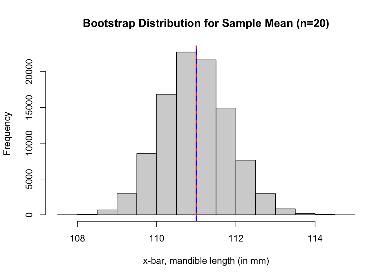
Solution to Question 8
Replace the ?? in the code cell below to calculate and store bootstrap estimate of bias to bias.jaw.
# calculate bootstrap estimate of bias
bias.jaw <- ??
bias.jaw  # print to screen
Question 9
Recall the data set environmental from the lattice package we worked with earlier to estimate the proportion of all time in New York City when the ozone concentration exceeds 70 ppb. In the code cell below, we load the lattice package and store the sample of ozone concentrations to a vector named nyc.oz.
Note
If you receive an error message when running the code cell below, then you do not have the lattice package installed.
- In the R console, run the command
install.packages("lattice"). - Then rerun the code cell below.
# be sure you have already installed the lattice package
library(lattice)  # loading lattice package
nyc.oz <- environmental$ozone  # store ozone data to a vector
The code cell below constructs a bootstrap distribution for the sample proportion of time the ozone concentration exceeds 70 ppb using the original sample nyc.oz. The corresponding bootstrap sample proportions are stored in the vector boot.prop.
- Read the code cell below.
- After interpreting the code, run the code cell. No edits are needed.
- In the code cell provided in the solution space, calculate the bootstrap estimate of bias.
Tip
In the case of bootstrap estimate for a proportion, we have \({\displaystyle\mbox{Bias}_{\rm{boot}} \big( \hat{p}_{\rm{boot}} \big) = {\color{dodgerblue}{\hat{p}_{\rm{boot}}}} - {\color{tomato}{\hat{p}}}}\).
##############################
# no edits needed
# read and run the code
#############################

N <- 10^5  # Number of bootstrap samples
boot.prop <- numeric(N)  # create vector to store bootstrap proportions
n.oz <- length(nyc.oz)

# for loop that creates bootstrap dist
for (i in 1:N)
{
  x <- sample(nyc.oz, size = n.oz, replace = TRUE)  # pick a bootstrap resample
  boot.prop[i] <- sum(x > 70)/n.oz  # compute bootstrap sample proportion
}

# plot bootstrap distribution
hist(boot.prop,
     breaks=20,
     xlab = "p-hat, sample proportion",
     main = "Bootstrap Distribution for Sample Proportion")

# bootstrap mean and standard error
boot.prop.mean <- mean(boot.prop)  # mean of bootstrap dist
boot.prop.se <- sd(boot.prop)  # SE of bootstrap dist

# red line at the observed sample proportion
abline(v = sum(nyc.oz > 70)/n.oz, col = "firebrick2", lwd = 2, lty = 1)
# blue line at the center of bootstrap dist
abline(v = boot.prop.mean, col = "blue", lwd = 2, lty = 2)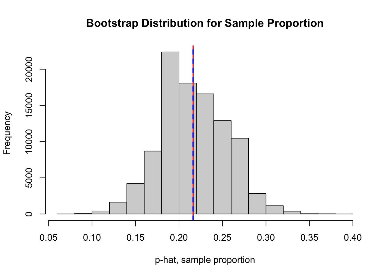
Solution to Question 9
Replace the ?? in the code cell below to calculate and store bootstrap estimate of bias to bias.ozone.
# calculate bootstrap estimate of bias
bias.ozone <- ??
bias.ozone  # print to screen
Question 10
Recall the data set birthwt from the MASS package we worked with earlier. In the code cell below, we load and clean the data in birthwt.
Note
If you receive an error message when running the code cell below, then you do not have the MASS package installed.
- In the R console, run the command
install.packages("MASS"). - Then rerun the code cell below.
library(MASS)  # load MASS package
birthwt$smoke[birthwt$smoke == 0]  <- "no"  # non-smokers assigned "no"
birthwt$smoke[birthwt$smoke == 1]  <- "smoker"  # smokers assigned "smoker"
birthwt$smoke <- factor(birthwt$smoke)  # convert smoke variable to categorical factor

# subset the sample into two independent samples
non <- subset(birthwt, smoke == "no")
smoker <- subset(birthwt, smoke == "smoker")
The code cell below constructs a bootstrap distribution for the difference in two sample means using the independent samples stored in the data frames non and smoker. The corresponding bootstrap difference in sample means are stored in the vector boot.dom.
- Read the code cell below.
- After interpreting the code, run the code cell. No edits are needed.
- In the code cell provided in the solution space, calculate the bootstrap estimate of bias.
##############################
# no edits needed
# read and run the code
#############################

N <- 10^5  # Number of bootstrap samples
boot.dom <- numeric(N)  # create vector to store bootstrap proportions

m.non <- length(non$bwt)
n.smoker <- length(smoker$bwt)

# for loop that creates bootstrap dist
for (i in 1:N)
{
  x.non <- sample(non$bwt, size = m.non, replace = TRUE)  # pick a bootstrap resample
  x.smoker <- sample(smoker$bwt, size = n.smoker, replace = TRUE)  # pick a bootstrap resample
  boot.dom[i] <- mean(x.non) - mean(x.smoker)  # compute difference in sample means
}

# plot bootstrap distribution
hist(boot.dom,
     breaks=20,
     xlab = "x.bar.non - x.bar.smoker (in grams)",
     main = "Bootstrap Distribution for Difference in Means")

# bootstrap mean and standard error
boot.dom.mean <- mean(boot.dom)  # mean of bootstrap dist
boot.dom.se <- sd(boot.dom)  # SE of bootstrap dist

# red line at the observed  difference in sample means
abline(v = mean(non$bwt) - mean(smoker$bwt), col = "firebrick2", lwd = 2, lty = 1)

# blue line at the center of bootstrap dist
abline(v = boot.dom.mean, col = "blue", lwd = 2, lty = 2)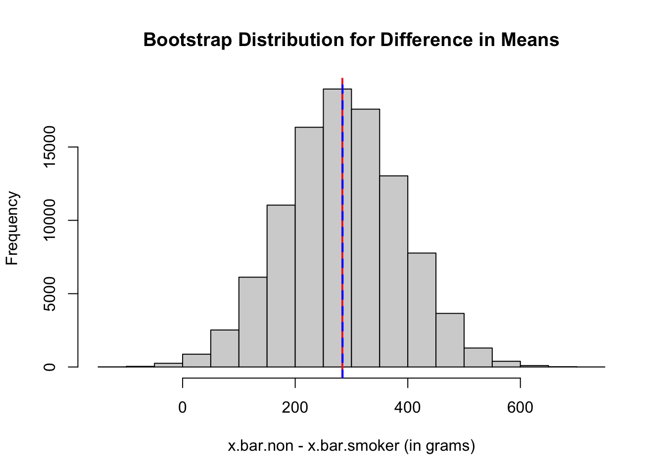
Solution to Question 10
Replace the ?? in the code cell below to calculate and store bootstrap estimate of bias to bias.smoke.
# calculate bootstrap estimate of bias
bias.smoke <- ??
bias.smoke  # print to screen
Question 11
Out of the three bootstrap estimates of bias in Question 8, Question 9, and Question 10, which bias is the most extreme?
Solution to Question 11
Rule of Thumb for Acceptable Bias
What is a significant amount of bias? The answer to this question does not depend on the bootstrap estimate of bias alone. We need to consider how much bias is present relative to the overall variability in sample statistics. For example:
- If the bootstrap estimate of bias is \(5\) and \(\mbox{SE}_{\rm{boot}} = 5,\!000\), then relatively speaking the bias is quite small.
- If the bootstrap estimate of bias is \(-0.1\) and \(\mbox{SE}_{\rm{boot}} = 2\), then relatively speaking the bias is much larger.
- We compare the value of the bootstrap estimate of bias relative to the bootstrap standard error.
- In the first example, we have the ratio \(\frac{5}{5000} = 0.001\).
- In the second example, we have a ratio \(\frac{-0.1}{2} = -0.05\)
- In general, we use the ratio of the bootstrap bias to the bootstrap standard error to measure how significant is the bias.
\[{\color{dodgerblue}{\boxed{ \mbox{Relative Bootstrap Bias} = \dfrac{\mbox{Bootstrap Bias}}{\mbox{Bootstrap SE}}}}}\]
Rule of Thumb for Bootstrap Bias
If either
\[{\color{dodgerblue}{\frac{\mbox{Bootstrap Bias}}{\mbox{Bootstrap SE}} > 0.02 \qquad \mbox{or} \qquad \frac{\mbox{Bootstrap Bias}}{\mbox{Bootstrap SE}} < -0.02,}}\]
then the bias is large enough to have a substantial effect on the accuracy of the estimate.
Question 12
Determine whether the jackal mandible bootstrap distribution in Question 8, the ozone concentration bootstrap distribution for sample proportion in Question 9, or the bootstrap distribution for the difference in mean birth weights Question 10 exceed the 0.02 rule of thumb. Relatively speaking, which of the three biases is most extreme?
Solution to Question 12

Statistical Methods: Exploring the Uncertain by Adam Spiegler is licensed under a Creative Commons Attribution-NonCommercial-ShareAlike 4.0 International License.