2.4: Common Discrete Distributions

In statistics, we are typically using data from a sample to make inferences about characteristics of a population. We want to may have claims or questions to test. We may want to estimate some characteristics or parameters of the population. By identifying patterns in the sample data and applying probability, we can build theoretical models to inform predictions about the population. These predictions depend on the level of uncertainty due to sampling, that may be flawed, biased, or simply unlikely. Data and models come in all shapes and levels of complexity.

We will take a look at several of the most common and useful distributions when working with discrete random variables, such as counting the frequency of occurrences in certain classes of categorical variables. There are many more distributions for discrete random variables, some of which we will see later!

A Case Study in Randomness: Jury Duty

Illustration by Eric Molinsky from the CALI Lesson “Trial Practice, Bringing it to the Jury and Beyond.” CC BY-NC-SA 2.0

The jury plays the most crucial role in a trial. They determine how cases are ultimately resolved! The jury serves as an impartial reviewer of the facts presented in criminal and civil cases. The goal of randomly selecting the jury is to remove the bias in the jury selection process.

How can we measure whether a jury that has been selected is “representative”?

A random sample of 12 adults cannot be a perfect representative of the population in all ways. No two distinct random samples of 12 adults is going to be same, yet we hope different juries would rule similarly based on the same set of facts if they are truly impartial. The jury system plays a vital role in the system of justice in the United States, and randomness plays a central role in helping reduce bias in court rulings.

How Jurors Are Selected

The federal judicial branch in the United States decides the constitutionality of federal laws and resolves disputes about federal laws. The federal court system is divided into 94 district courts. The US District Court in the District of Colorado randomly selects jurors from voter registration lists, driver license records, and state-issued adult identification records, by a computerized method. Below is an explanation of how juries are chosen in the District of Colorado. See The District of Colorado Juror Information for full details.

“This selection process creates the court’s ‘Master Jury Wheel’. (This term originated in the days when names were placed into a large barrel-type wheel and turned around to mix them up. Today, computers are used to select names randomly.) From the ‘Master Jury Wheel’, jurors are randomly selected for a one month term of service or occasionally longer depending on the court’s jury needs.”

Question 1

Consider the selection of a jury of 5 people. We want to see whether the jury is representative in terms of political party. Note we initially choose a jury of 5 people to more quickly recognize a pattern. After identifying a pattern, we can extend our results to juries of 12 people. Let \(Y\) denote a jury member who identifies as an independent voter. Let \(N\) denote a jury member who is not independent (identify as Democrat, Republican, or with another political party).

There is one possible outcome in the event: 0 people on the jury identify an Independent.
We can represent that outcome as NNNNN.

Question 1a

List all possible outcomes in the event: Exactly 1 out of 5 jurors is independent.

Solution to Question 1a

Question 1b

List all possible outcomes in the event: Exactly 2 out of 5 jurors are independent.

Solution to Question 1b

Counting Outcomes

Consider a district with \(n\) people eligible for jury duty. On the first of each month the court chooses a new pool of \(k\) people from which juries will be selected. How many different jury pools of size \(k\) can be selected from a population with size \(n\)?

There are \(n\) possible people that can be chosen first.
Then there are \(n-1\) remaining possible people that can be selected as person 2.
Then there are \(n-2\) remaining possible people that can be selected as person 3.
And so until there are \(n-(k-1)\) remaining people to select person \(k\).

\[\begin{array}{lclclcccl} \mbox{choice 1} & & \mbox{choice 2} & & \mbox{choice 3} & & & & \mbox{choice k} \\ n & \times & (n-1) & \times & (n-2) & \times & \ldots & \times & (n-(k-1)) \end{array} = \frac{n!}{(n-k)!}.\]

Note the factorial of a non-negative integer \(n\) is denoted \(\color{dodgerblue}{n!}\) and is the product of all positive integers less than or equal to \(n\):

\[\color{dodgerblue}{n! = 1 \times 2 \times 3 \times \ldots \times (n-1) \times n}\]

Ignoring the Order of Selection: N Choose K

If we want to count the total number of possible jury pools, and we do not care about the order in which the people are selected, then we want to count the number of combinations.

First count the possible outcomes as we illustrated above, taking into account the order in which the jury is selected.
Then we ignore the order that people are selected by considering the same set of people (chosen in any order) as the same. Using the result that there are \(k!\) ways of permuting the order of the \(k\) people selected.

Thus, the number of combinations of \(k\) items out of a set of \(n\), denoted \(_nC_k\) also referred to as \(n\) choose \(k\), is

\[\color{dodgerblue}{\begin{pmatrix} n \\ k \end{pmatrix} = \frac{n!}{k! (n-k)!}.}\]

Note

See the Appendix: Why Divide By \(k!\) if you are curious why we divide by \(k!\) when we do not care about the order that the items are selected.

Question 2

Use R to calculate the total number of outcomes in the event: Exactly 2 out of 5 jurors are independent voters.

Tip

The function factorial(x) calculates \(x!\) for a non-negative integer \(x\).

Solution to Question 2

# solution using factorial(x)

Tip

An Even Better Tip: The function choose(n, k) calculates \(\begin{pmatrix} n \\ k \end{pmatrix}\) for non-negative integers \(n\) and \(k\).

# solution using choose(n, k)

Defining a Random Variable

Recall random variables map outcomes in a sample space to a subset of the real numbers. In this example, an outcome is 5 randomly selected people for the jury. We define random variable \(X\) to be the number of independent voters on a randomly selected jury of 5 people. For example, we have:

The outcome NNNNN is mapped to \(X=0\).
The outcome YNNNN is mapped to \(X=1\).
The outcome NNNYN is also mapped to \(X=1\).
The outcome YNNYN is mapped to \(X=2\).

We map each outcome to an integer \(X\), and then we can compute values of the corresponding probability mass function (pmf) \(p(x) = P(X=x)\).

Question 3

According to a recent article “Why Independent Voters Are Key To Winning Colorado”, PBS News. Oct 3, 2020, approximately 42% of Colorado’s voters identify as independent.

In solving Question 2, there is a general pattern we can model to compute the probability of choose exactly \(x\) jurors that identify as an independent voters in a jury of 5 people. In this question, we generalize the pattern to answer questions about a jury of 12 people.

Question 3a

What is the probability of randomly selecting a jury of 12 people with exactly 0 jurors that identify as an independent voter?

Solution to Question 3a

# Use R to help compute P(X=0)

Question 3b

What is the probability of randomly selecting a jury of 12 people with exactly 1 juror that identify as an independent voter?

Solution to Question 3b

# Use R to help compute P(X=1)

Question 3c

What is the probability of randomly selecting a jury of 12 people with exactly 2 jurors that identify as independent voters?

Solution to Question 3c

# Use R to help compute P(X=2)

Question 3d

What is the probability of randomly selecting a jury of 12 people with at most 2 jurors that identify as independent voters?

Solution to Question 3d

# Use R to help compute probability X is at most 2

Question 3e

What is the probability of randomly selecting a jury of 12 people with at least 2 jurors that identify as independent voters?

Solution to Question 3e

# Use R to help compute probability X is at least 2

Question 4

A jury of 12 people is randomly selected from a population that is 42% independent voters. Let random variable \(X\) denote the number of jurors that identify as an independent voter.

Question 4a

Using your answers to Question 3, give the values for \(p(0)=P(X=0)\), \(p(1)=P(X=1)\), \(p(2)=P(X=2)\), and \(F(2) = P(X \leq 2)\).

Solution to Question 4a

\(p(0)=\) ??
\(p(1)=\) ??
\(p(2)=\) ??
\(F(2)=\) ??

Question 4b

Give a possible formula for the pmf of \(X\), \(p(x)=P(X=x)\).

Solution to Question 4b

A formula has been partially completed. Fill in the missing parts.

\[P(X=x) = \begin{pmatrix} ?? \\ ?? \end{pmatrix} (0.42)^{??} (1-0.42)^{??}\]

The Binomial Distribution

A Trial with Two Possible Outcomes

A Bernoulli trial is an experiment that has exactly two possible outcomes:

The probability that the outcome of a trial is a success (\(\color{dodgerblue}{X=1}\)) is denoted \(\color{dodgerblue}{p}\).
Otherwise, the probability of a failure (\(\color{tomato}{X=0}\)) is \(\color{tomato}{q=1-p}\).
\(X\) has a Bernoulli Distribution with probability mass function

\[f(x) = \left\{ \begin{array}{ll} p^x(1-p)^{1-x} & \mbox{for } x \in \left\{ 0, 1 \right \} \\ 0 , & \mbox{otherwise} \end{array} \right.\]

A Formula for the Binomial Distribution

Let random variable \(X\) be the number of successes out of \(n\) trials, where each trial is identical and independent.

\(X\) has a Binomial Distribution, written \(\color{dodgerblue}{X \sim \mbox{Binom}(n,p)}\).
The probability mass function is

\[f(x) = \left\{ \begin{array}{ll} \left( \begin{array}{c} n\\ x \end{array} \right) p^x(1-p)^{n-x} & \mbox{for } x =0,1,2, \ldots , n \\ 0 & \mbox{otherwise} \end{array} \right. \]

Note

See Appendix: Typsetting Arrays in LaTeX for more information on how to typeset formulas such as the piecewise function above using LaTeX.

Expected Value and Variance of Binomial Distributions

The expected value can be calculated with the shortcut \(\color{dodgerblue}{E(X) = np}\).
The variance can be calculated with the shortcut \(\color{dodgerblue}{\mbox{Var}(X) = np(1-p) = npq}\).

Binomial Distribution Functions in R

In R, the we can use the functions:

dbinom(x, n, p) calculates the probability of exactly \(x\) successes out \(n\) trials, \(\color{dodgerblue}{p(x)=P(X=x)}\).
pbinom(x, n, p) calculates the probability of at most \(x\) successes out \(n\) trials, \(\color{tomato}{F(x)=P(X \leq x)}\).
rbinom(m, n, p) randomly sample \(m\) values from \(X \sim \mbox{Binom}(n, p)\) (with replacement).
qbinom(q, n, p) compute the q^th quantile.

Plotting a Binomial Distribution

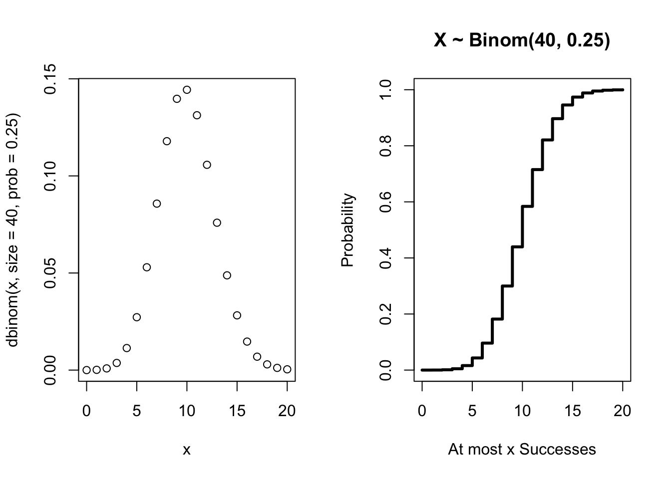
The figure below gives the graphs of the pmf and cdf for a binomial distribution with \(n=40\) and \(p = 0.25\).

Question 5

Suppose a manufacturer of electronic chargers knows that 5% of the chargers it produces are defective. The manufacturer sends a shipment of 20 randomly selected chargers to a customer. Write an R command to compute the probability of each event.

Question 5a

All 20 chargers sent are good (not defective).

Solution to Question 5a

# solution to 5a

Question 5b

At most 18 batteries are good.

Solution to Question 5b

# solution to 5b

Question 5c

At most 2 batteries are defective.

Solution to Question 5c

# solution to 5c

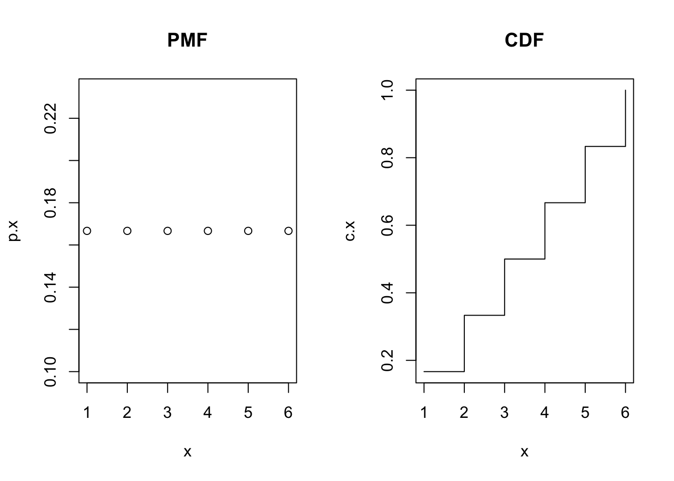
The Discrete Uniform Distribution

Question 6

Let \(X\) be the value of the result of rolling a fair six-sided die.

Question 6a

Write out the probability mass function \(f(x)\).

Solution to Question 6a

\[f(x) = \left\{ \begin{array}{ll} ?? & x = 1, 2, 3, 4, 5, 6 \\ 0 & \mbox{otherwise} \end{array} \right.\]

Question 6b

What is the expected value of rolling a fair-six sided die?

Solution to Question 6b

Question 6c

What is the expected value of rolling a fair die with sides \(1, 2, 3, \ldots , k\)?

Tip

Recall the sum of the first \(k\) integers is \(\displaystyle \sum_{n=1}^k n = \frac{k(k+1)}{2}\).

Solution to Question 6c

Note

See Appendix: The Discrete Uniform Distribution for a summary of key formulas, graphs, shortcuts, and R functions for working with a Discrete Uniform Distribution.

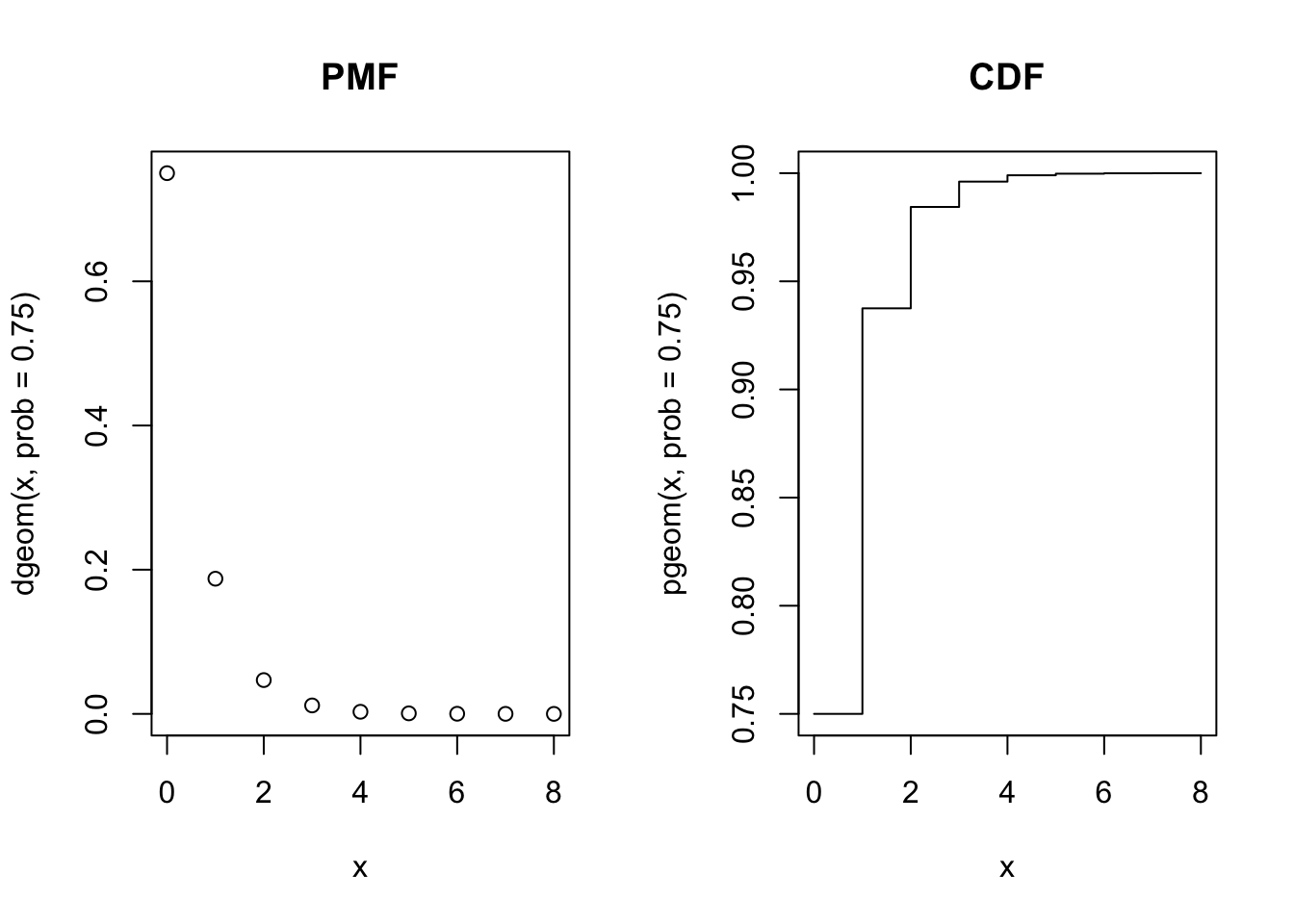
The Geometric Distribution

If we repeat a Bernoulli trial that has probability of success \(p\) for each trial, we can count the number of failures, \(X\), that occur before the first success. In such cases, \(X\) follows a geometric distribution, and we write \(\color{dodgerblue}{X \sim \mbox{Geom}(p)}\).

\[f(x) = q^xp \quad \mbox{for } x = 0, 1, 2, \ldots .\]

Note

See Appendix: The Geometric Distribution for a summary of key formulas, graphs, shortcuts, and R functions for working with a Geometric Distribution.

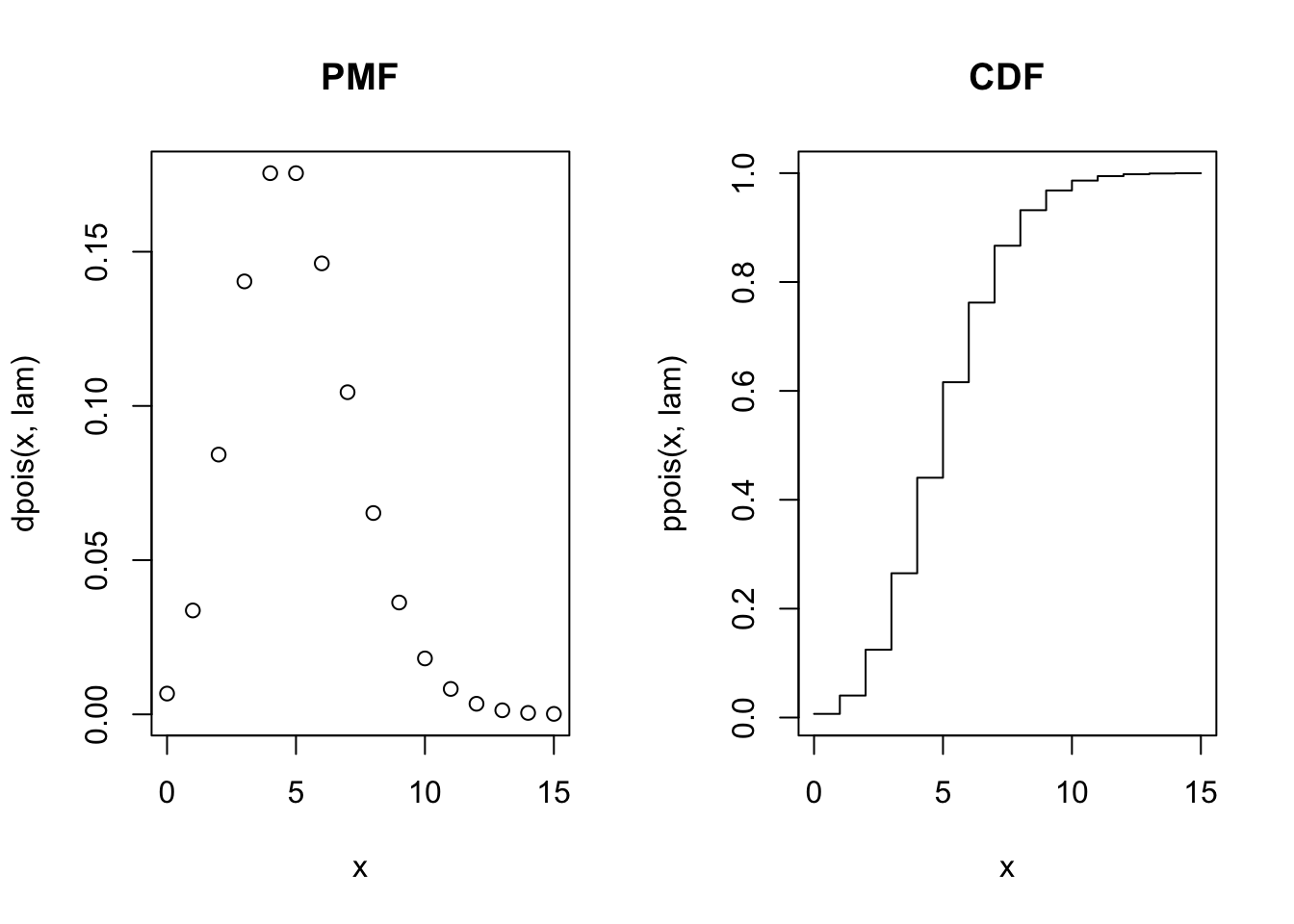
The Poisson Distribution

The Poisson distribution applies when the average frequency of occurrences in a given time period is known to be \(\lambda\), and each occurrence is independent of the others. Let \(X\) denote the number of times an event occurs in the given time period, then we have \(\color{dodgerblue}{X \sim \mbox{Pois}(\lambda)}\).

Note

See Appendix: The Poisson Distribution for a summary of key formulas, graphs, shortcuts, and R functions for working with a Poisson Distribution.

Practice with Discrete Random Variables

For each situation, identify which distribution best describes the distribution of the random variable. Then calculate the probability.

Question 7

A sports marketer for the Denver Nuggets randomly calls people in the Denver area until they encounter someone who attended a Nuggets game last season. Suppose we know that 10% of the population attended a Nuggets game last season, and we consider a call to a person who did attend a game last season as a success. What is the probability that the marketer has their first success on their eighth call?

Solution to Question 7

# solution to question 7

Question 8

Suppose we know that on average twelve cars cross a certain bridge each minute during rush hour. Find the probability that seventeen or more cars cross the bridge during a one minute span of time in rush hour.

Solution to Question 8

# solution to question 8

Question 9

Recently, a nurse commented that when a patient calls the medical advice line claiming to have the flu, the chance that he or she truly has the flu (and not just a nasty cold) is only about 4%. Of the next 25 patients calling in claiming to have the flu, what is the probability that exactly 4 patients will have the flu?

Solution to Question 9

# solution to question 9

Question 10

A online retailer sells an average of 5 big screen TV’s on a given day. What is the probability they sell 9 TV’s in a day?

Solution to Question 10

# solution to question 10

Question 11

It is known that 3% of airbags manufactured by a certain car company are defective. What is the probability that the first defective air bag occurs when the fifth item is inspected?

Solution to Question 11

# solution to question 11

Appendix A: Summary of Common Discrete Random Variables

The Binomial Distribution

\(X \sim \mbox{Binom}(n,p)\) is number of successes from \(n\) identical and independent trials each with probability of success \(p\).

\[f(x; n, p) = \left\{ \begin{array}{ll} \left( \begin{array}{c} n\\ x \end{array} \right) p^x(1-p)^{n-x} \ \ & \mbox{for } x =0,1,2, \ldots , n\\ & \\ 0 \ \ & \mbox{otherwise} \end{array} \right.\]

The expected value is \(E(X) = \mu_X = np\).
The variance is \(\mbox{Var} (X) = \sigma_X^2 = np(1-p)\).
Use dbinom(x, n, p) to calculate \(p(x) = P(X = x)\).
Use pbinom(x, n, p) to calculate \(F(x) = P(X \leq x)\).
Use rbinom(m, n, p) to generate a random sample of size \(m\) from population \(X \sim \mbox{Binom}(n,p)\).
Use qbinom(q, n, p) to find the q^th percentile of \(X \sim \mbox{Binom}(n,p)\).

The Discrete Uniform Distribution

There are \(k\) distinct outcomes each with an equal likelihood of occurring.

\[f(x; k) = \left\{ \begin{array}{ll} \dfrac{1}{k} \ \ & \mbox{for } x = 1, 2, \ldots, k\\ 0 \ \ & \mbox{otherwise} \end{array} \right.\]

The expected value is \(\displaystyle E(X) = \mu_X = \frac{k+1}{2}\).
The variance is \(\displaystyle \mbox{Var} (X) = \sigma_X^2 = \frac{k^2-1}{12}\).
Note functions such as dunif(), punif(), runif(), and qunif() are for the continuous (not discrete) uniform distribution.
It is typically easier to calculate probabilities directly rather than use technology.

The Geometric Distribution

\(X \sim \mbox{Geom}(p)\) is the number of failures that occur before the first success, where \(p\) denotes the probability of a success and \(q=1-p\) is the probability of a failure.

\[f(x; p) = \left\{ \begin{array}{ll} q^xp \ \ & \mbox{for } x = 0, 1, 2, \ldots \\ 0 & \mbox{otherwise} \end{array} \right. .\]

The expected value is \(E(X) = \mu_X = \dfrac{q}{p}\).
The variance is \(\mbox{Var} (X) = \sigma_X^2 = \dfrac{q}{p^2}\).
Use dgeom(x, p) to calculate \(p(x) = P(X = x)\).
Use pgeom(x, p) to calculate \(F(x) = P(X \leq x)\).
Use rgeom(m, p) to generate a random sample of size \(m\) from population \(X \sim \mbox{Geom}(p)\).
Use qgeom(q, p) to find the q^th percentile of \(X \sim \mbox{Geom}(p)\).

The Poisson Distribution

\(X \sim \mbox{Pois}(\lambda)\) is the number of times an event occurs in a fixed time period, where \(\lambda\) denotes the mean number of occurrences in the given time period.

\[f(x; \lambda) = \left\{ \begin{array}{ll} e^{-\lambda} \dfrac{\lambda^x}{x!} \ \ & \mbox{for } x = 0, 1, 2, \ldots \\ 0 & \mbox{otherwise} \end{array} \right. .\]

The expected value is \(E(X) = \mu_X = \lambda\).
The variance is \(\mbox{Var} (X) = \sigma_X^2 = \lambda\).
Use dpois(x, lambda) to calculate \(p(x) = P(X = x)\).
Use ppois(x, lambda) to calculate \(F(x) = P(X \leq x)\).
Use rpois(m, lambda) to generate a random sample of size \(m\) from population \(X \sim \mbox{Pois}(\lambda)\).
Use qpois(q, lambda) to find the q^th percentile of \(X \sim \mbox{Pois}(\lambda)\).

Appendix B: Additional Notes

Why Divide By \(k!\)?

Where does \(k!\) possible ways of permuting the order come from?

The symmetric group \(\color{dodgerblue}{S_k}\) on \(k\) items consists of all the possible ways of permuting the order of the \(k\) items.
Each element corresponds to a permutation applied to the group of \(k\) items.
For example \(S_3\) is the symmetric group on three items.
- The identity element is \((1,2,3)\) which does not change the ordering of items \(1, 2, 3\).
- The element \((1, \color{tomato}{3}, \color{tomato}{2})\) is the transpose of items 2 and 3.
- The element \((3, 1, 2)\) is a composition of two transpositions: - First transpose items 1 and 2, that is element \((\color{tomato}{2}, \color{tomato}{1}, 3)\). - Then transpose items 1 and 3 to get \((\color{tomato}{3}, 1, \color{tomato}{2})\).
The number of elements in the group is called the order of the group and denoted \(\color{dodgerblue}{|S_k|}\).
For example, \(S_3\) has \(|S_3|=6=3!\) elements that can be represented as

\[(1,2,3), (1,3,2), (2, 1, 3), (2, 3, 1), (3, 2, 1), \mbox{ and } (3, 1, 2).\]

In fact, for any symmetric group we have \(\color{dodgerblue}{|S_k|=k!}\).
Thus, there are \(k!\) ways of permutating the order of \(k\) items.

Typsetting Arrays in LaTeX

The array environment is started with \begin{array}.
Next we indicate how many columns and how each column is aligned.
- {ll} means two columns aligned to the left.
- {lrc} would be three columns: the first aligned left, then right, then the last column is centered.
- We use the & symbol to indicate a column break.
- We use \\ to indicate a row break.
If we want a big curly brace on the left of the array, enter \left\{ before beginning the array.
We do not want a brace on the other side of the array, so we use \right. to close off the left brace without using any matching symbol on the right.
We use \mbox{otherwise} to type the text otherwise inside the equation.

Creative Commons License

Statistical Methods: Exploring the Uncertain by Adam Spiegler is licensed under a Creative Commons Attribution-NonCommercial-ShareAlike 4.0 International License.