5.1: Bootstrap Distributions

Monte — Credit: Lévy et Neurdein réunis, Public domain, via Wikimedia Commons

Sampling From a Population

Rarely, we have access to data from the entire population of interest, in which case we are able to calculate the actual value(s) of population parameter(s). We can generate a sampling distribution by simulating the selection of many different random samples from the population data, and we can compute the standard error of the sampling distribution to measure how much uncertainty we can expect due to the randomness of sampling. If we have access to data from the entire population, there is no need for statistics to estimate parameters since we know the values of the parameters! Recall the distinction and connection and between parameters and statistics:

A parameter is a characteristic of a population (which may be a probability distribution).
- The values of population parameters are unknown, but their values are fixed and not random.
A statistic is a characteristic of a sample that we can use to approximate a parameter.
- Statistics are not fixed values. They will vary due to the randomness of sampling.
Recall we use different notation for parameters and statistics.
- We typically use \(\theta\) to denote a generic population parameter.
- We use hat notation, \(\color{dodgerblue}{\hat{\theta}}\), to denote estimators of \(\theta\).

In some situations, we have a known probability distribution that we can use to build a model and make predictions. For example, characteristics such as height (normal), time between successive events (exponential), and counting the number of times an event occurs over an interval of time all behave predictably (Poisson). We can pick random sample and use point estimators such as MLE and MoM to estimate unknown population parameters. What happens if the data does not follow a known distribution?

Suppose we would like to estimate the value of a parameter for a population about which we know very little information (this is often the case). We collect data from a single random sample of size \(n\), and then we can use statistics from the sample to make predictions about the population:

To estimate a population mean, it makes practical and mathematical sense to use a sample mean.
To estimate a population proportion, the sample proportion is an unbiased estimator.
To estimate a population variance, we can use the unbiased estimator \(s^2 = \frac{1}{n-1} \sum_{i=1}^n (x_i - \bar{x})^2\).

In any of these cases, how certain can/should we be in our estimate? In practice, we do not repeatedly pick 1000’s of random samples from the population. That is likely impractical, expensive, and time consuming. We have only collected data from a single random sample.

How can we account for the uncertainty in our estimate if we only have one random sample?

Question 1

Golden Jackal Portrait — Credit: Вых Пыхманн, CC BY-SA 3.0, Wikimedia Commons

Wolf and Jackal Mandible Bones — Credit: Вых Пыхманн, CC BY-SA 3.0, Wikimedia Commons

A zoologist would like to answer the following question:

What is the average mandible (jaw) length of all golden jackals (Canis aureus)?

Devise a method for collecting and analyzing data to help them answer this question.

Solution to Question 1

Case Study: Golden Jackal Mandible Length

The data frame¹ jackal in the permute package contains a sample of \(n=20\) mandibles from male and female golden jackals. For each of the 20 observations, two variables are recorded:

Length is the length of the mandible in millimeters (mm).
Sex is a categorical variable with two levels: Male and Female.

Loading the Data

It is very likely you do not have the package permute installed. You will need to first install the permute package.

Go to the R console window.
Run the command > install.packages("permute").

You will only need to run the install.package() command one time. You can now access permute anytime you like! However, you will need to run the command library(permute) during any R session in which you want to access data from the permute package. Be sure you have first installed the permute package before executing the code cell below.

# be sure you have already installed the permute package
library(permute)  # loading permute package

Summarizing and Storing the Data

In the code cell below we load the jackal data from the permute package and provide a numerical summary of the two variables in the sample.

data(jackal)  # load jackal data
summary(jackal)  # numerical summary of each variable

     Length          Sex    
 Min.   :105.0   Male  :10  
 1st Qu.:107.8   Female:10  
 Median :111.0              
 Mean   :111.0              
 3rd Qu.:113.2              
 Max.   :120.0

The code cell below displays the distribution of mandible lengths separately for males and females.

# side by side box plots
plot(Length ~ Sex, data = jackal, 
     col = c("dodgerblue", "mediumseagreen"),
     main = "Mandible Length of Golden Jackals",
     ylab = "Length (in mm)")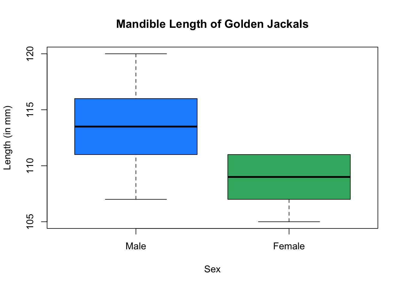

We will be analyzing mandible lengths for both adult male and female golden jackals. In the code cell below, we save the \(n=20\) mandible lengths to a vector called jaw.sample.

jaw.sample <- jackal$Length  # store mandible lengths to vector
jaw.sample  # print sample to screen

 [1] 120 107 110 116 114 111 113 117 114 112 110 111 107 108 110 105 107 106 111
[20] 111

Question 2

Based on the sample above, what is your estimate for \(\mu\), the mean mandible length of all adult golden jackals?

Solution to Question 2

# use jaw.sample to estimate population mean

Question 3

How much confidence do you have in your estimate in Question 2? Any suggestions on how we can measure the uncertainty in our estimate due to the randomness of sampling?

Solution to Question 3

What is a Statistical Question?

A statistical question is one that can be answered by collecting data and where there will be variability in that data.

Based on a random sample of \(n=20\) adult golden jackals, what is the mean mandible length of all adult golden jackals?

Each time we pick a different sample we have a different subset of data.
Different samples have different sample means, leading to different estimates.
This is a statistical question!
How can we account for this variability in our estimate?

Using a database that contains information on all registered voters in Colorado, what proportion of all Colorado voters are over 50 years old?

The database includes information from the population of all registered voters in Colorado.
We can use the population data to calculate the proportion.
The population data does not change, so there is no variability in the value of the proportion.
This is not an example of a statistical question.

Bootstrapping: Sampling from a Sample

We have explored the sampling distributions of sample means, proportions, medians, variances and other estimators as a tool to assess the variability in those statistics and measure the level of uncertainty or precision in the estimate we obtain from the sample. In particular, the variance of a sampling distribution or the standard error (which is the square root of the variance of a sampling distribution) are commonly used to assess the variability in sample statistics.

In the case of the mean mandible length of all golden jackals, we have collected one sample of \(n=20\) adult golden jackals. We do not have access to data from the entire population, so we cannot construct a sampling distribution by picking many different random samples each size \(n=20\). Collecting unbiased samples can be quite expensive, time-consuming, and logistically difficult. If we only have one sample and know very little about the population, how can we generate a sampling distribution from this limited information?

Bootstrap Distributions

Bootstrapping is the process of generating many different random samples from one random sample to obtain an estimate for a population parameter. For each randomly selected resample, we calculate a statistic of interest. Then we construct a new distribution of bootstrap statistics that approximates a sampling distribution for some sample statistic (such as a mean, proportion, variance, and others). We can use bootstrapping with any sample, even small ones. We can bootstrap any statistic. Thus, bootstrapping provides a robust method for performing statistical inference that we can adapt to many different situations in statistics and data science.

A Bootstrapping Algorithm

Given an original sample of size \(n\) from a population:

Draw a bootstrap resample of the same size, \(n\), with replacement from the original sample.
Compute the relevant statistic (mean, proportion, max, variance, etc) of that sample.
Repeat this many times (say \(100,\!000\) times).

A distribution of statistics from the bootstrap samples is called a bootstrap distribution.
A bootstrap distribution gives an approximation for the sampling distribution.
We can inspect the center, spread and shape of the bootstrap distribution and do statistical inference.

Question 4

Consider a random sample of 4 golden jackal mandible lengths (in mm):

\[120, 107, 110, \mbox{ and } 116.\]

Which of the following could be a possible bootstrap resample? Explain why or why not.

Question 4a

120, 107, 116

Solution to Question 4a

Question 4b

110, 110, 110, 110

Solution to Question 4b

Question 4c

120, 107, 110, 116

Solution to Question 4c

Question 4d

120, 107, 110, 116, 120

Solution to Question 4d

Question 4e

110, 130, 120, 107

Solution to Question 4e

Question 5

How many possible bootstrap resamples can be constructed from an original sample that has \(n=20\) values?

Solution to Question 5

# How many possible resamples are there for n=20?

Monte Carlo Methods

Monte Carlo methods are computational algorithms that rely on repeated random sampling. A bootstrap distribution is one example of a Monte Carlo method. A bootstrap distribution theoretically would contain the sample statistics from all possible bootstrap resamples. If we pick an initial sample size \(n\), then there exists a total of \(n^n\) possible bootstrap resamples. In the case of \(n=20\), we have \(20^{20} \approx 1.049 \times 10^{26}\) possible resamples. If we ignore the ordering in which we pick the sample, when \(n=20\), we have a total of \(68,\!923,\!264,\!410\) (almost 69 billion!) distinct bootstrap resamples.

For small samples, we could write out all possible bootstrap resamples. For larger values of \(n\) (and we see \(n=20\) is already extremely large), it is really not practical or feasible to generate all possible bootstrap resamples while avoiding duplicates. Instead, we use Monte Carlo methods to repeatedly pick random samples that we use to approximate a sampling distribution. The Monte Carlo method of generating many (but necessarily all) bootstrap resamples introduces additional uncertainty and variability into the analysis. The more bootstrap resamples we choose, the less uncertainty we have.

By default, we will create \(N =100,\!000 = 10^5\) bootstrap resamples.
In some cases (very large \(n\)), we may choose a smaller number of resamples for the sake of time.
For typically bootstrapping, it is recommended to use at least \(N=10,\!000\) bootstrap resamples.

Monte Carlo methods were first explored by the Polish mathematician Stanislow Ulam in the 1940s while working on the initial development of nuclear weapons at Los Alamos National Lab in New Mexico. The research required evaluating extremely challenging integrals. Ulam devised a numerical algorithm based on resampling to approximate the integrals. The method was later named “Monte Carlo”, a gambling region in Monaco, due to the randomness involved in the computations.

Creating a Bootstrap Distribution in R

Let’s return to our statistical question:

What is the average mandible (jaw) length of all golden jackals?

We have already picked one random sample of \(n=20\) adult golden jackals. The mandible lengths of our sample are stored in the vector jaw.sample.

Step 1: Pick a Bootstrap Resample

We use the sample() function in R to pick a random sample of values out of the values in jaw.sample.

Notice the resample has size \(n=20\), the same as the original sample.
We use the option replace = TRUE since we want to sample with replacement.
Running the code cell below creates one bootstrap resample stored in temp.samp.

temp.samp <- sample(jaw.sample, size=20, replace = TRUE)  # sample with replacement
temp.samp  # print sample to screen

 [1] 114 111 107 107 105 111 107 117 111 111 107 120 110 105 106 106 107 116 108
[20] 107

Step 2: Calculate Statistic(s) from the Bootstrap Sample

In the golden jackal mandible length example, we want to use information about the distribution of sample means to estimate a population mean. Thus, we calculate the mean of the bootstrap resample temp.samp that we picked in the previous code cell.

mean(temp.samp)  # mean of bootstrap resample

[1] 109.65

Step 3: Repeat Over and Over Again

In the code cell below, we repeat steps 1 and 2 over and over again. The sample means we calculate from each bootstrap resample are stored in a vector named boot.dist. Run the code cell below to generate a bootstrap distribution for the sample mean.

A solid red line marks the location of the sample mean from the original sample.
A dashed blue line marks the location of the mean of the bootstrap distribution.
A solid green line marks the location of another published estimate for the population mean².

##########################
# cell is ready to run
# no need for edits
##########################
N <- 10^5  # Number of bootstrap samples
boot.dist <- numeric(N)  # create vector to store bootstrap means

# for loop that creates bootstrap dist
for (i in 1:N)
{
  x <- sample(jaw.sample, 20, replace = TRUE)  # pick a bootstrap resample
  boot.dist[i] <- mean(x)  # compute mean of bootstrap resample
}

# plot bootstrap distribution
hist(boot.dist,  
     breaks=20, 
     xlab = "x-bar, mandible length (in mm)",
     main = "Bootstrap Distribution for Sample Mean (n=20)")

# red line at the observed sample mean
abline(v = mean(jaw.sample), col = "firebrick2", lwd = 2, lty = 1)

# blue line at the center of bootstrap dist
abline(v = mean(boot.dist), col = "blue", lwd = 2, lty = 2)

# green line at the population mean, 112 mm
abline(v = 112, col = "mediumseagreen", lwd = 2, lty = 1)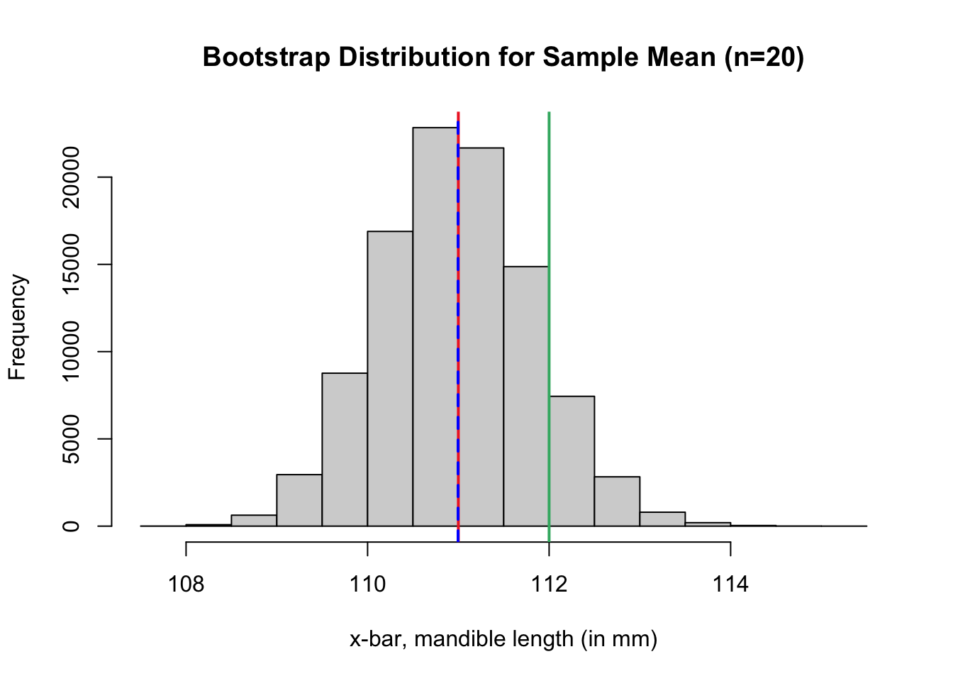

Question 6

What are the mean and standard error of the bootstrap distribution? Use the code below to compute each value.

# calculate center of bootstrap dist


# calculate bootstrap standard error

Solution to Question 6

Measuring the Bias of Booststrap Estimates

Recall if \({\color{tomato}{\widehat{\theta}}}\) is an estimator for the parameter \({\color{mediumseagreen}{\theta}}\), then we define the bias of an estimator as

\[{\large \color{dodgerblue}{ \boxed{\mbox{Bias}(\widehat{\theta}) = {\color{tomato}{E \left( \widehat{\theta} \right)}} - {\color{mediumseagreen}{\theta}}}.}}\]

In the case of bootstrapping:

We use the center of the bootstrap distribution, \({\color{tomato}{\hat{\mu}_{\rm{boot}}}}\), as the bootstrap estimator.
We use the mean from the original sample, \({\color{mediumseagreen}{\bar{x}}}\), in place of the parameter \(\theta\).
We define the bootstrap estimate of bias as

\[{\large \color{dodgerblue}{ \boxed{\mbox{Bias}_{\rm{boot}} \big( \hat{\mu}_{\rm{boot}} \big) = {\color{tomato}{\hat{\mu}_{\rm{boot}}}} - {\color{mediumseagreen}{\bar{x}}}.}}}\]

Caution

When estimating a population mean, we use the center of the bootstrap distribution, \({\color{tomato}{\hat{\mu}_{\rm{boot}}}}\) as the estimator for the population mean.

Do not use the mean of the original sample, \(\bar{x}\), as the estimator.
The values of \(\hat{\mu}_{\rm{boot}}\) and \(\bar{x}\) are usually very close, but not equal.
The difference \(\hat{\mu}_{\rm{boot}} - \bar{x}\) is used to estimate the bias of \(\hat{\mu}_{\rm{boot}}\).

Question 7

Compute the bootstrap estimate of bias if we use the mean of the bootstrap distribution from Question 6 as our estimate for the mean mandible length of all adult golden jackals.

Solution to Question 7

Question 8

What common distribution do you believe is the best model for mandible lengths of all golden jackals? Explain your reasoning.

Solution to Question 8

A Central Limit Theorem Model

Let \(X\) be the mandible length (in mm) of a randomly selected adult golden jackal. Based on the sample data in jaw.sample, we could come up with unbiased estimates for the population mean and population variance using:

\(\mu \approx \hat{\mu} = \frac{1}{n} \sum x_i =\) mean(jaw.sample) \(=111\) mm.
\(\sigma^2 \approx s^2 = \frac{1}{n-1} \sum (x_i - \bar{x})^2 =\) var(jaw.sample) \(=15.05\) mm².
This gives \(\sigma \approx s = \sqrt{15.05} = 3.88\) mm.

We now have an estimate for the population, namely \(X \sim N(111, 3.88)\). We can apply the Central Limit Theorem (CLT) for Means to construct another estimate for the sampling distribution. Although our sample size is relatively small (\(n=20 < 30\)), we can apply CLT in this situation since the population is assumed to be symmetric (normally distributed).

Question 9

Using the CLT with the population model \(X \sim N(111, 3.88)\), we can derive a theoretical model for the distribution of sample means for \(n=20\). Using the CLT for means, give the mean and standard error for the sampling distribution for \(\overline{X}\). How do your answers compare to approximations you found in Question 6 using the bootstrap distribution to estimate the sampling distribution for sample means?

Solution to Question 9

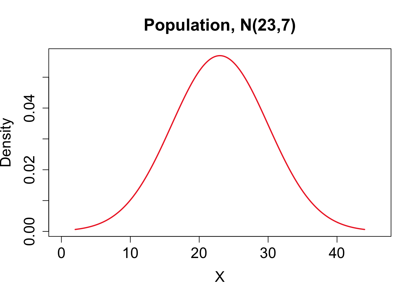
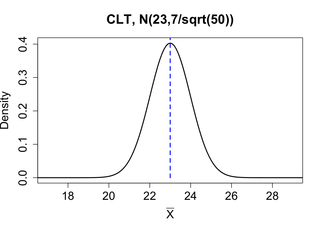
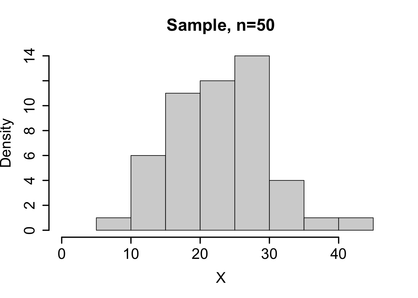
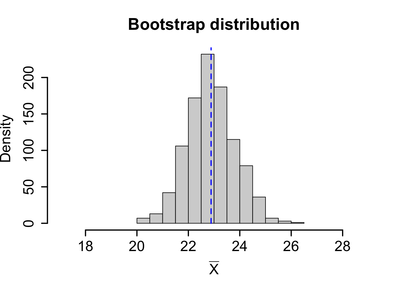
Comparison of Bootstrap Approximations to CLT

Consider the theoretical population \(X \sim N(23,7)\). Below we compare the sampling distribution for the mean obtained using the central limit theorem on the top row with one random sample and a corresponding bootstrap distribution for the sample mean on the bottom row.

	Mean	Standard deviation.
Population	\(\mu_X= 23\)	\(\sigma_X = 7\)
Theoretical Sampling Dist for \(\overline{X}\)	\(\mu_{\bar{X}}= 23\)	\(\sigma_{\overline{X}} = \mbox{SE}(\overline{X}) = 0.99\)
Sample (\(n=50\))	\(\bar{x} = 22.69\)	\(s = 6.15\)
Bootstrap distribution	\(\hat{\mu}_{\rm{boot}} = 22.88\)	\(\mbox{SE}_{\rm{boot}}(\overline{X}) = 0.938\)

Question 10

Compare the population and sample distributions. What is similar about the two distributions? What are the differences?

Compare the CLT sampling distribution and bootstrap sampling distribution. What is similar about the two distributions? What are the differences?

Solution to Question 10

Solution to part a:

Solution to part b:

The Plug-in Principle

The Plug-in Principle: If something (such as a characteristic of a population) is unknown, substitute (plug-in) an estimate. For example, if we do not know the population mean \(\mu\), the sample mean \(\bar{x}\) is a nice, unbiased substitute. If a population standard deviation \(\sigma\) is unknown, we can use substitute the sample standard deviation, \(s\).

Bootstrapping is an extreme application of this principle.
We replace the entire population (not just one parameter) by the entire set of data from the sample.

Each bootstrap resample is picked from the same “population”, the original sample, to generate a bootstrap distribution that can be used to estimate a sampling distribution constructed from the entire population.

Properties of Bootstrap Estimators

The goal of a bootstrap distribution is to estimate a sampling distribution for some statistic.
Bootstrap distributions are biased estimators for a population mean since they are centered near \(\bar{x}\) not necessarily \(\mu\).
- Thus, the mean of a bootstrap distribution is not useful alone.
- But bootstrapping is useful at quantifying the behavior of a parameter estimate.
For most common statistics, bootstrap distributions provide good estimates for the true spread, shape, and bias of a sampling distribution for the statistic of interest.

Question 11: Arsenic Case Study

Arsenic is a naturally occurring element in the groundwater in Bangladesh. Much of this water is used for drinking in rural areas, so arsenic poisoning is a serious health issue. The data set Bangladesh in the resampledata package³ contains measurements on arsenic, chlorine, and cobalt levels (in parts per billion, ppb) present in each of 271 groundwater samples.

Loading the Data

It is very likely you do not have the package resampledata installed. You will need to first install the resampledata package.

Go to the R console.
Run the command > install.packages("resampledata").

You will only need to run the install.package() command one time. You can now access resampledata anytime you like! However, you will need to run the command library(resampledata) during any R session in which you want to access data from the resampledata package. Be sure you have first installed the resampledata package before executing the code cell below.

# be sure you have already installed the resampledata package
library(resampledata)  # loading resampledata package

Question 11a

Complete the code cell below to calculate the mean and standard deviation and size of the arsenic level of the sample.

Solution to Question 11a

# be sure you have already installed the resampledata package
arsenic <- Bangladesh$Arsenic  # store arsenic data in vector
n.arsenic <- length(arsenic)  # how many observations in arsenic

################################
# complete each command below
################################
mean.arsenic <- ??  # sample mean
sd.arsenic <- ??  # sample standard deviation
mean.arsenic  # print result to screen
sd.arsenic  # print result to screen

Question 11b

Create a histogram to show the shape of the distribution of the sample data. How would you describe the shape?

Solution to Question 11b

# create a histogram of the sample arsenic data
hist(??)

Question 11c

Complete the code cell below to generate a bootstrap distribution for the sample mean. What are the mean and standard error of the bootstrap distribution?

Solution to Question 11c

Replace all eight ?? in the code cell below with appropriate code. Then run the completed code to generate a bootstrap distribution.

N <- 10^5  # number of bootstrap samples
boot.arsenic <- numeric(N)  # create vector to store bootstrap means

# Set up a for loop!

for (i in 1:N)
{
  x <- sample(??, size = ??, replace = ??)  # pick a bootstrap resample
  boot.arsenic[i] <- ??  # calculate relevant sample statistic
}

boot.mean <- mean(??)  # calculate center of bootstrap dist
boot.se <- sd(??)  # calculate bootstrap standard error

# plot bootstrap distribution
hist(boot.arsenic,  xlab = "xbar",
     main = "Bootstrap Distribution")

# add a red line at the observed sample mean
abline(v = ??, col = "firebrick2", lwd = 2, lty = 1)

# add a blue line at the center of bootstrap dist
abline(v = ??, col = "blue", lwd = 2, lty = 2)

# print bootstrap estimate and standard error to screen
boot.mean  # mean (center) of bootstrap dist
boot.se  # standard error (spread) of bootstrap dist

# compare bootstrap dist to normal dist
# run to create a qq-plot
qqnorm(boot.arsenic)
qqline(boot.arsenic)

Question 11d

Calculate the bootstrap estimate for bias.

Solution to Question 11d

# calculate bootstrap estimate of bias

Creative Commons License

Statistical Methods: Exploring the Uncertain by Adam Spiegler is licensed under a Creative Commons Attribution-NonCommercial-ShareAlike 4.0 International License.

Manly, B.F.J. (2007) Randomization, bootstrap and Monte Carlo methods in biology. Third Edition. Chapman & Hall/CRC, Boca Raton.↩︎
Ali Louei Monfared, “Macro-Anatomical Investigation of the Skull of Golden Jackal (Canis aureus) and its Clinical Application during Regional Anesthesia”, Global Veterinaria 10 (5): 547-550, 2013.↩︎
Laura M. Chihara and Tim C. Hesterberg (2019) Mathematical Statistics with Resampling and R. Second Edition. John Wiley & Sons, Hoboken, NJ.↩︎