library(dplyr)
population <- storms$wind5.4: Parametric Confidence Intervals for Means
![]()
Parametric and Non-Parametric Methods
We have been investigating resampling methods as a tool to estimate the variability in sample statistics. Statistics such as means and proportions are linear combinations of random variables, and using theory from probability, we are able the derive the Central Limit Theorem (CLT) formulas to model sampling distributions for means and proportions. In this section we will construct confidence intervals by applying a parametric approach that uses formulas from the CLT to measure the uncertainty (standard error) in our estimate.
- With parametric methods, we perform inference using formulas derived from theory to model the shape, center and spread of sampling distributions.
- Monte Carlo methods such as bootstrap resampling are non-parametric since they use simulations to estimate sampling distributions.
Note
For statistics that are not linear combinations of independent random variables (such as medians, variances, and ratios of means) deriving formulas to model the sampling distribution is more complicated or not even possible. We can try bootstrapping in these situations instead!
Case Study: Average Wind Speed of Storms

Suppose a climatologist has contacted us for help estimating the average wind speed of all storms in the North Atlantic. They have collected a random sample of \(n=36\) wind speeds from North Atlantic storms over the past 5 years.
Loading Storms Data
When practicing exploratory data analysis earlier, we accessed the dplyr package that contains a data set from the NOAA Hurricane Best Track Data, called storms, with data on many different storm attributes. We will begin analyzing the variable wind that gives the wind speed in knots. Run the code cell below to:
- Load the
dplyrpackage (which should already be installed), and - Store the wind speeds to a new vector called
population.
Note
If you receive an error message when running the code cell below, then you may not have the dplyr package installed.
- In the R console, run the command
install.packages("dplyr"). - Then rerun the code cell below.
Picking a Random Sample of Storms
When performing statistical inference, we do not have complete data from the entire population. We typically have data from one sample picked randomly from the population. Based on the sample data, we try to estimate unknown parameters for the population. To begin our exploration of confidence intervals, suppose the 19066 wind speeds in the population data represents the full population of all storms at all times in the North Atlantic. We investigate the following statistical question:
What is the average wind speed of all storms in the North Atlantic, \(\mu_{\rm{wind}}\)?
- Assume we do not have access to all the
populationdata and cannot directly calculate \(\mu_{\rm{wind}}\). - We will pick one random sample of 36 wind speeds from the
population. - We will use our sample to estimate the mean wind speed of all storms in the North Atlantic.
Question 1
Pick a random sample of \(n=36\) wind speeds from the population. In picking your original sample, sample without replacement. Store your sample to a vector named my.sample.
Solution to Question 1
# pick one random sample of 36 wind speeds without replacement
my.sample <- sample(??, size = ??, replace = ??)
Question 2
Using the random sample my.sample, give a possible point estimate for \(\mu_{\rm{wind}}\), the mean wind speed of all storms in the North Atlantic. The parameter \(\mu_{\rm{wind}}\) is unknown since we assume the full population data is not available.
Solution to Question 2
# use your sample to give a point estimate
A Bootstrap Confidence Interval
Before introducing parametric methods for constructing a confidence interval estimate, we first review resampling methods to construct a bootstrap distribution from the sample my.sample that we can use to construct a bootstrap confidence interval. The code below uses the original sample my.sample to generate a bootstrap distribution for the sample mean wind speed (with \(n=36\)) that is stored in boot.wind for the next step.
Note
If you are not familiar with bootstrapping methods, but you would like to learn more about parametric methods, feel free to jump to the next section on parametric methods.
N <- 10^5  # Number of bootstrap samples
boot.wind <- numeric(N)  # create vector to store bootstrap means
n <- 36  # sample size

# for loop that creates bootstrap dist
for (i in 1:N)
{
  x <- sample(my.sample, size = n, replace = TRUE)  # pick a bootstrap resample
  boot.wind[i] <- mean(x)  # compute bootstrap sample mean
}

boot.wind.est <- mean(boot.wind)  # mean of bootstrap dist
boot.wind.se <- sd(boot.wind)  # bootstrap standard error
my.mean <- mean(my.sample)  # original sample mean
In the code cell below, we use the bootstrap sample means (stored in boot.wind above) to construct a 95% bootstrap percentile confidence interval estimate for the mean wind speed of all North Atlantic storms.
lower.boot.wind <- quantile(boot.wind, 0.025)  # lower 95% cutoff
upper.boot.wind <- quantile(boot.wind, 0.975)  # upper 95% cutoff

# print to screen
lower.boot.wind
2.5%
51.25 upper.boot.wind 97.5%
72.36111 Based on the output from the previous code cell, we have a 95% bootstrap percentile confidence interval for the mean wind speed of all North Atlantic storms, namely from 51.25 knots to 72.36 knots. Note the interval estimates may vary, so you likely have a slightly different interval estimate if you are working with a different sample.
In the code cell below, we plot the bootstrap distribution with the original sample mean of my.sample marked with a red vertical line and the cutoffs for the confidence interval marked with blue vertical lines.
#################################
# code is ready to run!
# no need to edit the code cell
#################################

# plot bootstrap distribution
hist(boot.wind,
     breaks=20,
     xlab = "x.bar, sample mean wind speed (in knots)",
     main = "Bootstrap Distribution for Sample Mean")

# red line at the observed sample proportion
abline(v = my.mean, col = "firebrick2", lwd = 2, lty = 1)

# blue lines marking cutoffs
abline(v = lower.boot.wind, col = "blue", lwd = 2, lty = 2)
abline(v = upper.boot.wind, col = "blue", lwd = 2, lty = 2)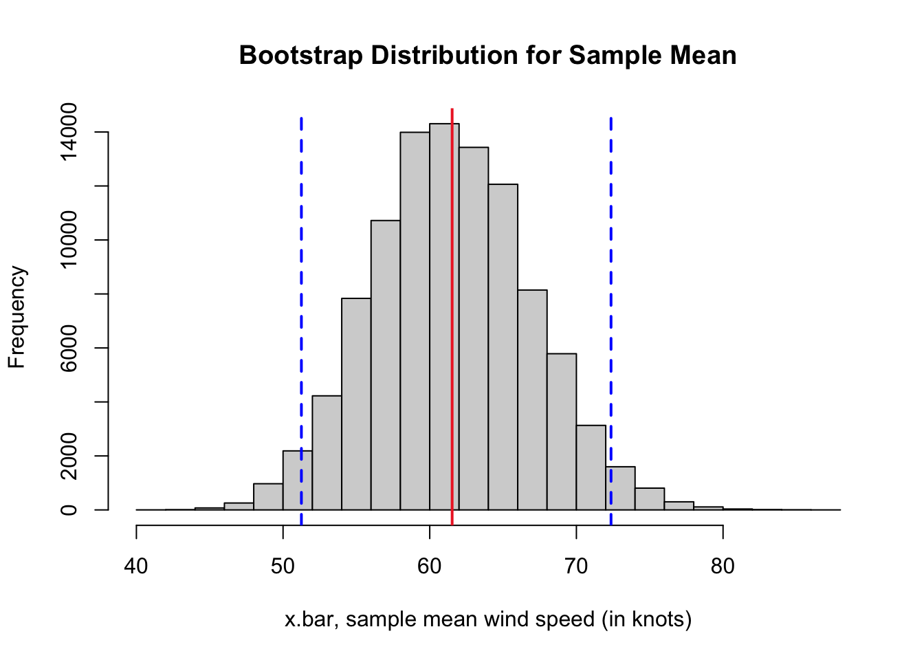
A Parametric Method for Interval Estimates
Recall the 68%-95%-99.7% empirical rule for normal distributions that states approximately:
- 68% of all values fall within one standard deviation (both above and below) from the mean.
- 95% of all values fall within two standard deviations of the mean.
- 99.7% of all values fall within three standard deviations of the mean.
Question 3
Check the accuracy of the empirical rule for normal distributions.
Question 3a
Using the R code cell below, check the accuracy of the approximation that 68% of the data is within \(\pm 1\) standard deviation from the mean.
Tip
Using the standard normal distribution \(Z \sim N(0,1)\), compute \(P(-1 < Z < 1)\).
Solution to Question 3a
# how much data is within +/- 1 standard deviation?
Question 3b
Using the R code cell below, check the accuracy of the approximation that 95% of the data is within \(\pm 2\) standard deviation from the mean.
Solution to Question 3b
# how much data is within +/- 2 standard deviations?
Question 3c
Using the R code cell below, check the accuracy of the approximation that \(99.7\)% of the data is within \(\pm 3\) standard deviation from the mean.
Solution to Question 3c
# how much data is within +/- 3 standard deviations?
Question 3d
Let’s improve the approximation that 95% of the data is withing \(\pm 2\) standard deviations from the mean. Find a more accurate approximation for \(z^*\) such that \(P( -z^* < Z < z^* ) = 0.95\).
Tip
Sketch a picture to help determine how much area is in the left tail below \(-z^*\) if 95% of the area is between \(-z^*\) and \(z^*\). Then use the qnorm() command.
Solution to Question 3d
# find more accurate cutoffs for the middle 95%
qnorm(??, 0, 1)
Question 4
Let \(X\) denote the wind speed of a randomly selected North Atlantic storm. We use \(\mu\) and \(\sigma\) to denote the mean and standard deviation, respectively, of the wind speed of the population of all storms in the North Atlantic. Answer the questions below to investigate a different approach to constructing an interval estimate for \(\mu\).
Question 4a
Let \(\overline{X}\) denote the distribution of sample means for samples size \(n\). Recall we denote the mean and standard error of the sampling distribution as \(\mu_{\overline{X}}\) and \(\sigma_{\overline{X}}\), respectively.
Justify each of the steps below.
\[\begin{aligned} 0.95 &= P \left( -1.96 < Z < 1.96 \right) & \mbox{from Question 3d}\\ 0.95 &= P \left( -1.96 < \frac{\overline{X} - \mu_{\overline{X}}}{\sigma_{\overline{X}}} < 1.96 \right) & \mbox{Explanation 1}\\ 0.95 &= P \left( -1.96 < \frac{\overline{X} - \mu}{\frac{\sigma}{\sqrt{n}}} < 1.96 \right) & \mbox{Explanation 2}\\ 0.95 &= P \left( -1.96 \cdot \frac{\sigma}{\sqrt{n}} < \overline{X}- \mu < 1.96 \cdot \frac{\sigma}{\sqrt{n}} \right) & \mbox{Explanation 3} \\ 0.95 &= P \left( - \overline{X} -1.96 \cdot \frac{\sigma}{\sqrt{n}} < - \mu < - \overline{X} + 1.96 \cdot \frac{\sigma}{\sqrt{n}} \right) & \mbox{Explanation 4} \\ 0.95 &= P \left( \overline{X} - 1.96 \cdot \frac{\sigma}{\sqrt{n}} < \mu < \overline{X}+1.96 \cdot \frac{\sigma}{\sqrt{n}} \right) & \mbox{Explanation 5}\\ \end{aligned}\]
Solution to Question 4a
Explanation 1:
Explanation 2:
Explanation 3:
Explanation 4:
Explanation 5:
Question 4b
Let \(\mu_{\rm{wind}}\) denote the mean wind speed of all North Atlantic storms which we assume is unknown. How can we use the result that \(P \left( \overline{X} - 1.96\cdot \sigma_{\overline{X}} < \mu_{\rm{wind}} < \overline{X}+1.96 \cdot \sigma_{\overline{X}} \right)=0.95\) to help construct a confidence interval for \(\mu_{\rm{wind}}\)?
Solution to Question 4b
Question 4c
You will use the original random sample of \(n=36\) wind speeds stored in my.sample in Question 1 to construct an interval estimate using the result from Question 4b. If you have not already loaded the population data and created a sample size \(n=36\) stored in my.sample, be sure to answer Question 1 before continuing. Create a histogram to display the wind speeds in my.sample.
Solution to Question 4c
# Enter code to create a histogram to display your sample
Question 4d
Are the assumptions for the CLT for means satisfied by the data in my.sample? Explain why or why not.
Solution to Question 4d
Question 4e
We assume the population data is unknown and we do not know the actual value of the parameter \(\mu_{\rm{wind}}\). However, suppose we do know the population variance \(\mbox{Var}(X) = \sigma^2_{\rm{wind}} = 650\) square knots. Using the CLT for means, what is the value of \(\sigma_{\overline{X}}\), the standard error of the sampling distribution for \(\overline{X}\)? Show your work below either doing calculations by hand or in R. Tip: In R, the square root function is sqrt().
Solution to Question 4e
# compute standard error using CLT
Question 4f
Give an interval of values \(?? < \mu_{\rm{wind}} < ??\) that has a 95% chance of containing the actual value of \(\mu_{\rm{wind}}\). Include supporting work/code to explain how you determined your answer.
Solution to Question 4f
# compute upper and lower cutoffs for interval estimate
95% Confidence Interval for a Mean
For a sample of size \(n\) randomly picked from a normal distribution with unknown \(\mu\) and known \(\mbox{Var}(X)=\sigma^2\), a 95% confidence interval for the mean is
\[{\color{dodgerblue}{\boxed{ \large \overline{X} - 1.96 \frac{\sigma}{\sqrt{n}} < \mu < \overline{X} + 1.96 \frac{\sigma}{\sqrt{n}}}}}.\]
If we draw 1000’s of random samples each size \(n\) from a normal distribution with parameters \(\mu\) and \(\sigma^2\) and compute a 95% confidence interval from each sample, then about 95% of the intervals would successfully contain \(\mu\). The 95% is the confidence level of the interval and gives the success rate of the interval estimate.
Question 5
A another climatologist collects their own random sample of \(n=36\) wind speeds of North Atlantic storms.
Question 5a
Pick their random sample (without replacement) of \(n=36\) wind speeds from the population. Store the other sample to a vector named their.sample.
Solution to Question 5a
# pick another random sample of 36 wind speeds without replacement
their.sample <- sample(??, size = ??, replace = ??)
Question 5b
Using the random sample their.sample, give a possible point estimate for \(\mu_{\rm{wind}}\), the mean wind speed of all storms in population.
Solution to Question 5b
# use their sample to give another point estimate
Question 5c
Are the two point estimates in Question 2 and Question 5b equal?
Solution to Question 5c
Question 5d
Are the true values of the population parameter different or the same for both climatologists?
Solution to Question 5d
Question 5e
Without checking, which point estimate (Question 2 or Question 5b) do you believe is “better”?
Solution to Question 5e
What is Uncertain and What is Unknown?
It can be easy to confuse the terms uncertain and unknown. In a less formal setting, people may use these terms interchangeably. In statistical inference, there is a clear distinction in their meaning that is important to clarify:
- Each sample statistic is a known value that is uncertain due to sampling.
- Each climatologist has a different sample.
- The sample means will be different for different researchers.
- The population parameter is an unknown value that is certain (not variable).
- The parameter we are trying to estimate is a fixed (certain) value.
- The value of the parameter is however unknown.
- Each climatologist has a different estimate but both are trying to hit the same fixed target.
- We cannot be certain whether our estimate is successful or not if \(\mu_{\rm{wind}}\) is unknown!
Interpreting Confidence Intervals
Question 6
A researcher collects a random sample of size \(n=36\) of wind speeds for storms in the North Atlantic and calculates a 95% confidence interval for the mean wind speed that is from \(48.75\) knots to \(65.41\) knots. For each statement, determine whether the interpretation is correct or not. If not, explain why not.
Question 6a
There is a 95% chance that a randomly selected storm in the North Atlantic has a wind speed between \(48.75\) and \(65.41\) knots.
Solution to Question 6a
Question 6b
There is a 95% chance that the mean wind speed of all storms in the North Atlantic is between \(48.75\) and \(65.41\) knots.
Solution to Question 6b
Question 6c
There is a 95% chance the interval from \(48.75\) to \(65.41\) knots contains the mean wind speed of all storms in the North Atlantic.
Solution to Question 6c
Question 6d
95% of all random samples of size \(n=36\) North Atlantic storms have a sample mean wind speed between \(48.75\) and \(65.41\) knots.
Solution to Question 6d
Question 6e
There is a 95% chance the interval from \(48.75\) to \(65.41\) knots contains the mean wind speed of a random sample of \(n=36\) storms.
Solution to Question 6e
Attaching Uncertainty to the Intervals
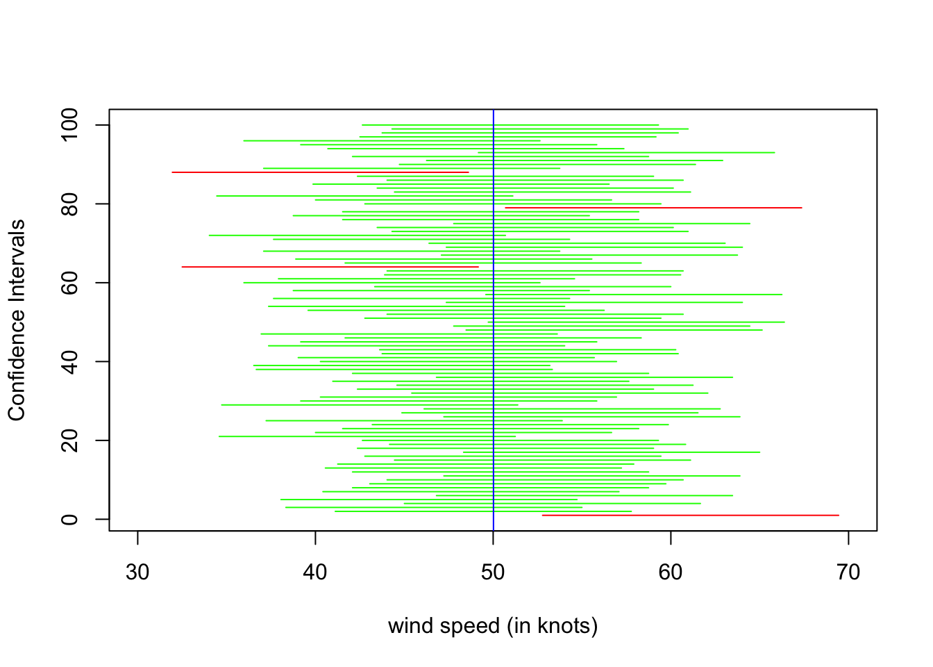
The plot shows 100 different confidence intervals based on 100 different random samples each size \(n=36\) storms selected from the population. For each sample mean \(\overline{X}\), we follow the same process of constructing a 95% confidence interval using:
\[\overline{X} - 1.96 \frac{\sigma}{\sqrt{n}} < \mu_{\rm{wind}} < \overline{X} + 1.96 \frac{\sigma}{\sqrt{n}}.\]
- Each sample results is a different interval estimate (all with the same width).
- The true population mean is marked with a blue vertical line at \(\mu_{\rm{wind}} = 50.02\) knots.
- The goal of each interval is to contain the same, fixed value of the population parameter.
- The confidence intervals that successfully contain \(\mu_{\rm{wind}} = 50.02\) are marked in green.
- The unsuccessful confidence intervals that do not contain \(\mu_{\rm{wind}} = 50.02\) are marked in red.
- 2 out of the 100 interval estimates are underestimates.
- 2 out of the 100 interval estimates are overestimates.
- We have a success rate of 96 out of 100 in this simulation.
- If we ran this simulation many more times, the success rate would converge to 95%.
Question 7
What are some warnings to keep in mind when interpreting confidence intervals?
Solution to Question 7
Warning 1:
Warning 2:
Warning 3:
Question 8
You will use the original random sample of \(n=36\) wind speeds stored in my.sample in Question 1 to construct a new confidence interval estimate for the mean wind speed of all North Atlantic storms. If you have not already loaded the population data and created a sample size \(n=36\) stored in my.sample, be sure to answer Question 1 before continuing.
Question 8a
Based on your sample data in my.sample, give a 90% confidence interval for the mean wind speed of all North Atlantic storms using the parametric method. As with earlier, suppose we know population variance is \(\sigma^2_X = 650\). Interpret the practical meaning of your 90% confidence interval in the context of this example.
Solution to Question 8a
new.z <- ??  # Enter a command to calculate z value for 90% Conf Level
wind.lower90 <- ??   # Enter a command to calculate the lower limit
wind.upper90 <- ??   # Enter a command to calculate the upper limit

# Print your answers
wind.lower90
wind.upper90
Practical interpretation of your 90% confidence interval:
Question 8b
As we decrease the confidence level of the interval from 95% in Question 4f to 90% in Question 8a, what happened to the width of the interval estimate?
Solution to Question 8b
Changing the Confidence Level
For a sample of size \(n\) randomly picked from a normal distribution with unknown \(\mu\) and known \(\mbox{Var}(X)=\sigma^2\), then a confidence interval for the mean is given by
\[\boxed{ \large \overline{X} - {\color{tomato}{z_{\alpha/2}}} \cdot \frac{\sigma}{\sqrt{n}} < \mu < \overline{X} + {\color{tomato}{z_{\alpha/2}}} \cdot \frac{\sigma}{\sqrt{n}}},\]
where the area under \(N(0,1)\) between \(\pm z_{\alpha/2}\) is equal to the confidence level of the estimate.
- The confidence level is the success rate of the estimate.
- The distance \({\color{dodgerblue}{\mbox{MoE} = z_{\alpha/2} \cdot \frac{\sigma}{\sqrt{n}}}}\) is called the Margin of Error (MoE) of the confidence interval.
\[\boxed{ \large \mu \approx \overline{X} \pm {\color{dodgerblue}{\mbox{MoE}}}}\]
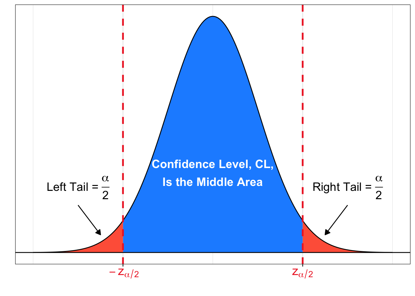
Let CL denote a selected confidence level that is the proportion of area in the middle.
- We have \({\color{mediumseagreen}{\alpha = 1 - CL}}\) is the area in the two tails.
- The area in each tail is therefore \(\color{tomato}{\dfrac{\alpha}{2}}\).
Confidence Intervals When the Variance Is Unknown
When estimating a population mean, in addition to \(\mu\) being unknown, we often do not know the population variance, \(\sigma^2\), either. We pick a random sample size \(n\), and we can plug-in the sample mean \(\bar{x}\) as our point estimate for \(\mu\). How can we find the margin of error if \(\sigma\) is unknown?
- We can use the sample standard deviation \(\color{tomato}{s}\) in place of \(\sigma\).
From the CLT for means, as long as the sample is normally distributed or if \(n \geq 30\), then we know the distribution of sample means \(\overline{X}\) is normally distributed with mean \({\color{mediumseagreen}{\mu_{\overline{X}} = \mu_X}}\) and standard error \({\color{dodgerblue}{\sigma_{\overline{X}} = \frac{\sigma}{\sqrt{n}}}}\). Thus, the standardized distribution of \(z\)-scores corresponding the sampling distribution for the sample mean \(\overline{X}\) is normal:
\[Z = \frac{\overline{X} - \color{mediumseagreen}{\mu_{\overline{X}}}}{{\color{dodgerblue}{\sigma_{\overline{X}}}}} = \frac{\overline{X} - \color{mediumseagreen}{\mu_{X}}}{{\color{dodgerblue}{\sigma_{X}/\sqrt{n}}}} \sim N(0,1).\]
Let’s apply our substitution of \(s\) in place of \(\sigma_{X}\) and consider the resulting distribution of standardized statistics denoted \(W\):
\[Z = \frac{\overline{X} - \mu_{X}}{{\color{tomato}{\sigma_{X}}}/\sqrt{n}} \quad \xrightarrow{\text{plug-in } {\color{tomato}{s}} \text{ for } {\color{tomato}{\sigma_{X}}}} \quad W = \frac{\overline{X}-\mu_X}{{\color{tomato}{s}}/\sqrt{n}} \sim \mbox{ ?}\]
- The plot on the left gives a histogram for the standardized sampling distribution \(W\).
- The plot on the right is a QQ-plot comparing the distribution of \(W\) to \(Z \sim N(0,1)\).
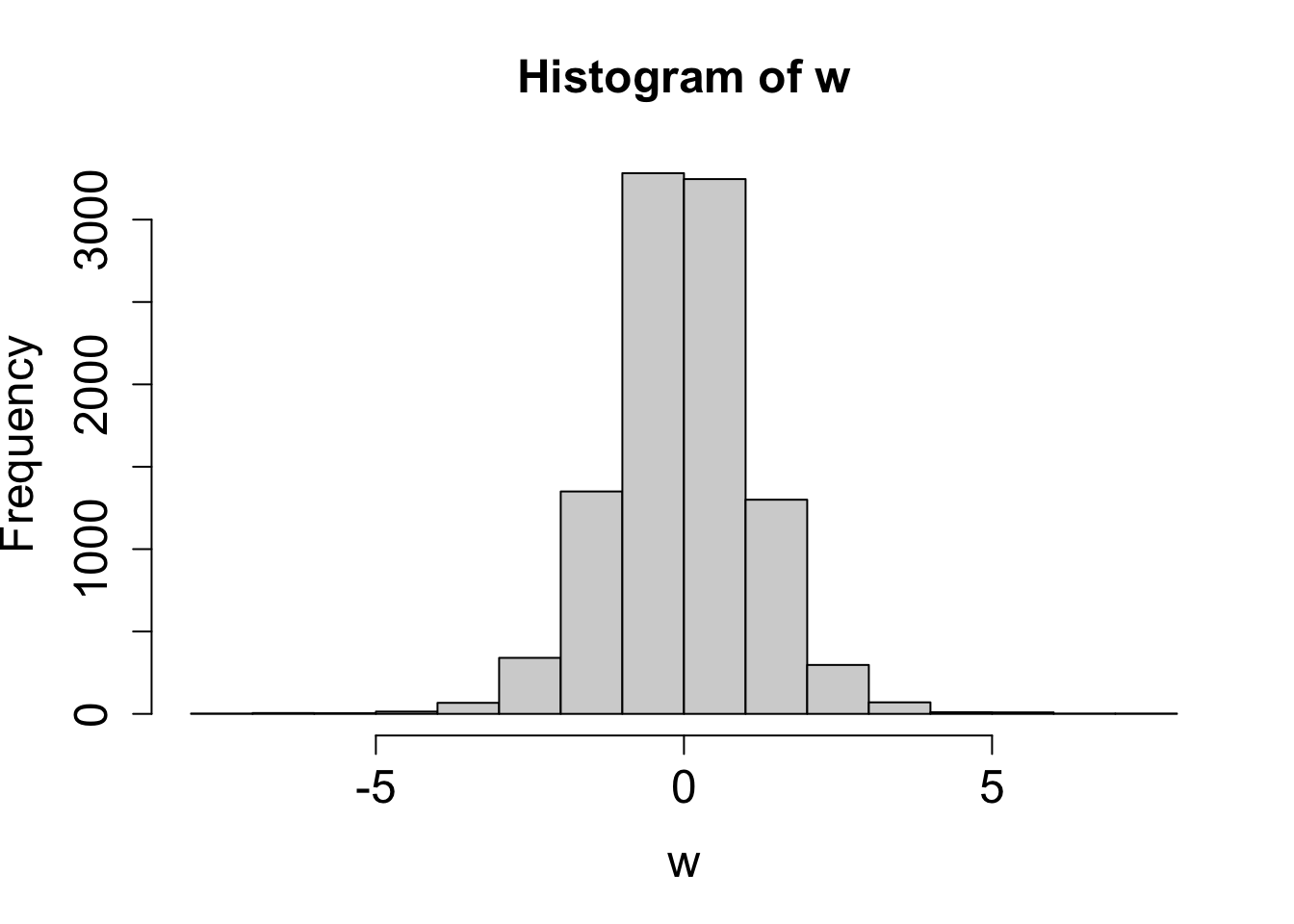
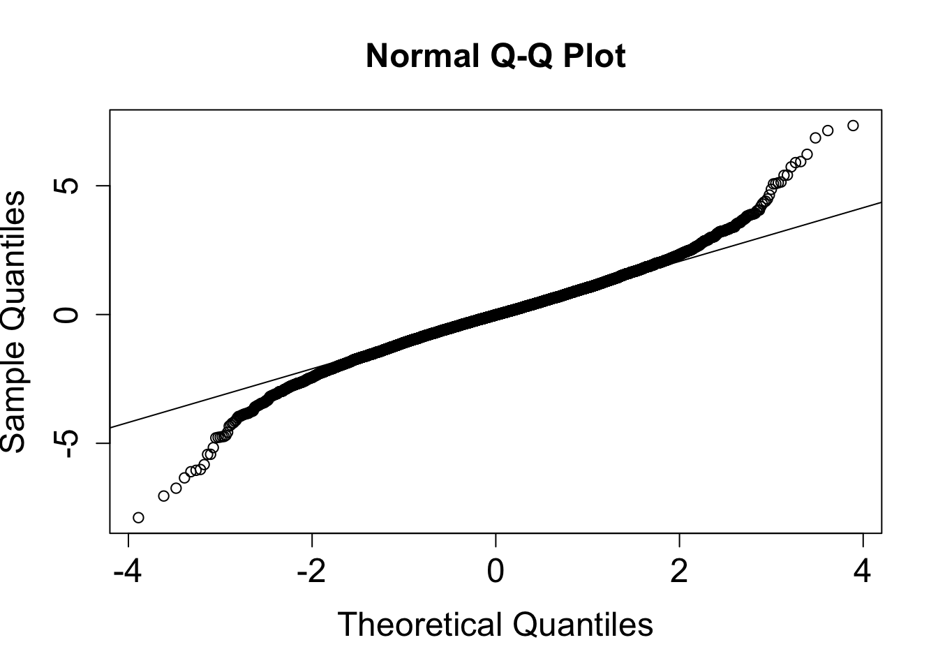
The distribution \(W\) is symmetric and bell-shaped. From the QQ-plot, we see \(W\) is approximately normal in the middle of the distribution. However, the tails of distribution \(W\) are not similar to tails of a normal distribution. Distribution \(W\) has fatter tails than a normal distribution.
- The fatter tails are due to the added uncertainty with using \(s\) to estimate the value of \(\sigma\).
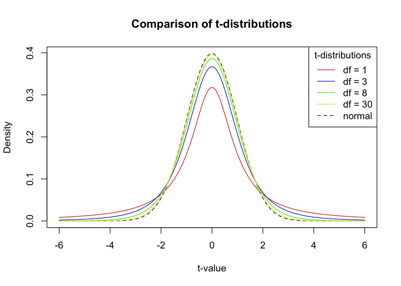
The \(t\)-Distribution
When the population is known to be normally distributed, the distribution \(W\) is a \(t\)-distribution with \(n-1\) degrees of freedom, where \(n\) denotes the sample size. If the underlying population is known to be symmetric (but not necessarily normal), a \(t\)-distribution with \(n-1\) degrees of freedom is still a good estimate.
- The larger our sample size \(n\), the better (less biased) the estimate \(s\) is for \(\sigma\).
- The larger the sample size \(n\), the closer the \(t\)-distribution is to \(Z \sim N(0,1)\).
If a random sample of data is skewed, then the population is likely skewed. The more skewed the population is, the less accurate a \(t\)-distribution is to estimate the distribution of the standardized statistic \(W\).
Warning
In cases where the sample is small (\(n < 30\)) and skewed, a bootstrap confidence interval is typically preferred to using a \(t\)-distribution to approximate the margin of error.
Using a \(t\)-Distribution When Variance is Unknown
For a sample of size \(n\) randomly picked from a normal distribution with unknown \(\mu\) and unknown \(\mbox{Var}(X)=\sigma^2\), we construct a confidence interval for \(\mu\) using:
- The sample standard deviation \(s\) in place of \(\sigma\), and
- A \(t\)-distribution to find \(t_{\alpha/2}\) instead of using \(N(0,1)\) to find \(z_{\alpha/2}\)
A corresponding \(t\)-distribution confidence interval is given by
\[{\large \boxed{ \overline{X} - {\color{dodgerblue}{t_{\alpha/2}}} \cdot \frac{{\color{tomato}{s}}}{\sqrt{n}} < \mu < \overline{X} + {\color{dodgerblue}{t_{\alpha/2}}} \cdot \frac{{\color{tomato}{s}}}{\sqrt{n}}}},\]
where the area under the \(t\)-distribution with \(n-1\) degrees of freedom between \({\color{dodgerblue}{\pm t_{\alpha/2}}}\) is equal to the confidence level.
Question 9

Researchers want to estimate the average length of all adult female Komodo dragons. The pick a random sample of \(n=8\) adult female Komodo dragons with the following weights (in pounds). They believe the distribution in weights will by normally distributed, but otherwise, the population variance is unknown.
dragon.wt <- c(145, 178, 142, 139, 160, 190, 168, 122)  # load sample of weights
dragon.wt  # print to screen
[1] 145 178 142 139 160 190 168 122Question 9a
Use the R code cell below to construct a 95% confidence interval for mean weight of all female Komodo dragons using the sample weights in dragon.wt.
Tip
Using the data in dragon.wt, calculate the statistics \(\bar{x}\) and \(s\). To find \(t_{\alpha/2}\), use the qt() function similar to how you use the qnorm() to calculate \(z_{\alpha/2}\). For more help using the qt() function, run ?qt().
Solution to Question 9a
# construct a 95% confidence interval
Question 9b
Interpret the practical meaning of the confidence interval in Question 9a in this context.
Solution to Question 9b
Question 9c
Use the R code cell below to construct a 99% confidence interval for mean weight of all female Komodo dragons using the sample weights in dragon.wt.
Solution to Question 9c
# construct a 99% confidence interval
Different Methods for \(t\)-Distribution Confidence Intervals
Use the formula \(\displaystyle \overline{X} - {\color{dodgerblue}{t_{\alpha/2}}} \cdot \frac{{\color{tomato}{s}}}{\sqrt{n}} < \mu < \overline{X} + {\color{dodgerblue}{t_{\alpha/2}}} \cdot \frac{{\color{tomato}{s}}}{\sqrt{n}}\).
- Use the
qt()function in R to find the value of \(t_{\alpha/2}\), or - Use a \(t\)-distribution table to estimate values for \(t_{\alpha/2}\).
- Use the
Use the R function
t.test(x, conf.level)$conf.int.xis the vector of sample data.- Set the confidence level with the
conf.leveloption. - Open the help manual with
?t.testfor further information.
Question 10
Using the Komodo dragon sample data in dragon.wt and the t.test() function, find a 95% confidence interval. Compare the results with the 95% confidence interval from Question 9a.
Solution to Question 10
t.test(??, conf.level = ??)$conf.intConfidence Interval for a Difference in Two Means
Question 11
Let \(X\) and \(Y\) be independent random variables with \(X \sim N(\mu_1, \sigma_1)\) and \(Y \sim N(\mu_2, \sigma_2)\). Using properties of expected value and variance, show for sample sizes \(n_1\) and \(n_2\), respectively, that
\[E(\overline{X}-\overline{Y}) = \mu_1-\mu_2 \qquad \mbox{and} \qquad \mbox{Var}(\overline{X}-\overline{Y}) = \frac{\sigma_1^2}{n_1} + \frac{\sigma_2^2}{n_2}.\]
Solution to Question 11
Confidence Intervals for a Difference in Means
Let \(X_1, X_2, \ldots , X_{n_1}\) be independent and identically distributed (i.i.d.) random variables picked from \(X \sim N(\mu_1, \sigma_1^2)\) and let \(Y_1, Y_2, \ldots , Y_{n_2}\) be i.i.d. random variables picked from \(Y \sim N(\mu_2, \sigma_1^2)\). An approximate confidence interval for the difference in means \(\mu_1 - \mu_2\) is given by:
\[{\large \boxed{ {\color{mediumseagreen}{(\overline{X} - \overline{Y})}} - {\color{tomato}{t_{\alpha/2}}} \cdot {\color{dodgerblue}{\sqrt{\frac{s_1^2}{n_1} + \frac{s_2^2}{n_2}}}} < \mu_1 - \mu_2 < {\color{mediumseagreen}{(\overline{X} - \overline{Y})}} + {\color{tomato}{t_{\alpha/2}}} \cdot {\color{dodgerblue}{\sqrt{\frac{s_1^2}{n_1} + \frac{s_2^2}{n_2}}}}}}. \]
- Use \(\bar{x} - \bar{y}\) as the point estimate for \(\mu_1 - \mu_2\).
- Approximate the standard error using \(s_1\) and \(s_2\) in place of unknown standard deviations \(\sigma_1\) and \(\sigma_2\).
- The area under the \(t\)-distribution with \(df\) degrees of freedom between \(\pm t_{\alpha/2}\) is equal to the confidence level.
- Informally, we can use the smaller of \(n_1-1\) and \(n_2-1\) as the degrees of freedom.
- Many R functions use the more accurate Welch’s approximation for the degrees of freedom,
- We do not need to memorize Welch’s approximation since
t.test()uses this method.
Which Month Has the Strongest Storms?
In our analysis of North Atlantic storm wind speeds, we used data stored in the storms data frame in the dplyr package. In our initial analysis, we assumed the data in storms represented the population, and we did not have access to the population data in storms. The data in storms is actually a sample of 19066 storm observations taken for North Atlantic storms that are measured every six hours during the lifetime of the storm. The population of interest is all storms that occur at all times in the North Atlantic.
- Consider data in
stormsas a random sample of 19066 observations picked from the population. - We have access to the sample
stormsthat we will use estimate parameters for the population. - Below, we load
dplyrand generate side-by-side box plots of the distribution of wind speeds in thestormssample by month.
library(dplyr)
storms$month <- factor(storms$month)  # convert month to categorical factor
boxplot(wind ~ month,
        data = storms,
        main = "Distribution of Wind Speeds by Month",
        xlab = "Month",
        ylab = "Wind speed (in knots)")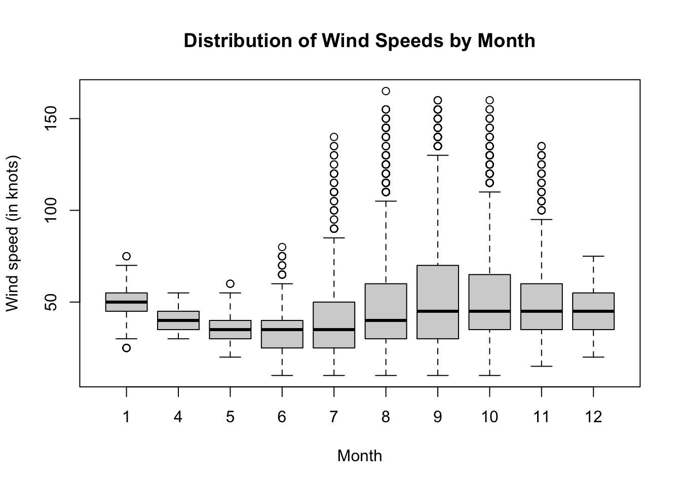
Question 12
Based on the plots in the figure above, in which month do you suspect storms have the greatest wind speed? Explain how you determined your answer.
Solution to Question 12
Refining Our Question
There are different statistics for assessing “greatest wind speed”. From the box plots, we have a good visual comparison of medians. With storms, outliers are typically the most important observations we do want to emphasize in our analysis. Thus, we use the mean as our measurement of center instead of a median or trimmed mean.
Side-by-side box plots give a nice graphical summary of the distribution of winds speeds by month. As we might suspect, from this first plot we rule out some months from this analysis. Some months appear to have very similar distributions upon inspection of box plots. We dig a little into the sample data to determine which months have the greatest sample mean wind speeds.
- We use the
tapply()function below to calculate and compare sample mean wind speeds by month. - Here is a nice introduction to the
tapply()function.
tapply(storms$wind, storms$month, mean) 1 4 5 6 7 8 9 10
49.85714 38.86364 35.17413 35.32092 41.39426 48.14414 54.56013 51.58109
11 12
49.42741 45.54245 Notice September (9) and October (10) are the two months with the highest mean wind speeds of \(54.56\) knots and \(51.58\) knots, respectively. The two means are close, and we only have a subset of population data. Is the observed difference in sample means greater than the margin of error we can expect due to the uncertainty of sampling? We can use a confidence interval to answer this question!
Give a 95% confidence interval to estimate the difference in the mean wind speed of storms in September compared to October?
Subsetting into Two Independent Samples
Run the code cell below to create two data frames, sep.wind and oct.wind, containing separate samples of wind speeds for North Atlantic storms in September and October, respectively. Both sep.wind and oct.wind are data frames with just one variable, wind.
# create a vector of sep wind
sep.wind <- subset(storms,
              month == "9",
              select = wind)

# create a vector of oct wind
oct.wind <- subset(storms,
              month == "10",
              select = wind)
Question 13
Answer the questions below to construct a 95% confidence interval for the difference in mean wind speeds of North Atlantic storms in September compared to October.
Question 13a
Calculate \(n_s\) and \(n_o\), the number of observations in September and October samples, respectively. Store the results in n.s and n.o.
Solution to Question 13a
# calculate n_s
n.s <- ??
# calculate n_o
n.o <- ??

# print to screen
n.s
n.o
Question 13b
Using the sample data in sep.wind and oct.wind, give a point estimate for the difference in population means, \(\mu_s - \mu_o\). Store the result to point.est
Solution to Question 13b
# calculate point estimate
point.est <- ??
point.est  # print to screen
Question 13c
Using a \(t\)-distribution, calculate the margin of error of a 95% confidence interval for the difference in means.
Tip
Use the sd() function to calculate each sample standard deviation. Use the qt() function to identify \(t_{\alpha/2}\) using the informal count for the degrees of freedom.
Solution to Question 13c
# use code cell to construct a 95% confidence intervalBased on the output above, a 95% confidence interval is from ?? to ??.
Question 13d
Interpret the meaning of your interval in Question 13c. In particular, can we conclude that wind speeds are on average greater in one month or the other?
Solution to Question 13d
Using t.test() for a Difference in Means
The t.test() function in R can used to construct a confidence interval for a difference in means from two independent populations using a \(t\)-distribution with Welch’s approximation for the degree’s for freedom. Let x and y denote vectors containing data from each of the two independent samples.
- The command
t.test(x, y, conf.level = 0.95)$conf.intwill give a 95% confidence level for the difference in means using Welch’s approximation.
Question 14
Use the t.test() function with the samples sep.wind and oct.wind to construct a 95% confidence interval for the difference in mean wind speeds of North Atlantic storms in September compared to October. How does your answer compare to your confidence interval in Question 13c? If the two answers are different, which confidence interval do you believe is more accurate?
Solution to Question 14
Complete the command below and then compare result to answer in Question 13c.
t.test(??, ??, conf.level = ??)$conf.int
Subsetting with t.test
Frequently, we would like to compare the distributions of a quantitative variable, denoted quant, for two different groups based on a categorical variable in the data set, denoted categorical. If our sample data is stored in a data frame called data.name with this structure, we can use t.test() without having to first split the sample into independent samples according to category group. t.test() can subset the data into independent samples for us and construct a confidence interval for the difference in two means. Using the t.test() function
t.test(quant ~ categorical, data = data.name, conf.level = 0.95)$conf.int
will give a 95% confidence level for the difference in means of a specified quantitative variable between the two different groups of the categorical variable.
Question 15
The code cell below subsets the sample data for all months in storms to a new data frame named pooled that:
- Includes only storm observations from September or October.
- Selects only two variables,
windandmonth, to keep fromstorms. - The first six rows of the data frame
pooledare printed to the screen withhead(pooled). - Run the code cell below and inspect the first six rows of
pooled.
pooled <- subset(storms,
               month == "9" | month == "10",   # month is 9 OR month is 10
               select = c(wind, month))  # select wind and month variables

head(pooled)  # print first 6 rows of pooled to screen
# A tibble: 6 × 2
wind month
<int> <fct>
1 30 9
2 20 9
3 20 9
4 75 9
5 75 9
6 75 9 Use the t.test() function with the pooled sample pooled to construct a 95% confidence interval for the difference in mean wind speeds of North Atlantic storms in September compared to October. How does your answer compare to your confidence intervals in Question 13c and Question 14? If the intervals are different, which confidence interval do you believe is most accurate?
Solution to Question 15
Complete the command below and then compare the result to your answers in Question 13c and Question 14.
t.test(?? ~ ??, data = ??, conf.level = ??)$conf.int
Caution Using t.test() for a Difference in Two Means
The variable month in the original sample storms has observations from 10 different months. If you try running the command t.test(wind ~ month, data = storms, conf.level = 0.95)$conf.int you will receive an error since the categorical variable month has more than two classes. The categorical variable used to split the data must have exactly 2 different classes. In solving Question 15 we avoided this error by:
- First creating the
pooledsample that included only two months, September and October. - Then using
t.test()with thepooledsample instead of the fullstormsdata set.
Otherwise, we can split the original sample into two independent samples x and y and use the t.test() function as we did in Question 14 with independent wind speed samples sep.wind and oct.wind.

Statistical Methods: Exploring the Uncertain by Adam Spiegler is licensed under a Creative Commons Attribution-NonCommercial-ShareAlike 4.0 International License.