bmi <- seq(26 - 4*4, 26 + 4*4, length=100)3.1: Sampling Distribution of Means
![]()
A sampling distribution is the distribution of sample statistics (such as a mean, proportion, median, maximum, etc.) computed for different samples of the same size from the same population. A sampling distribution shows us how much the sample statistic varies from sample to sample. The exercises in this section compare the sampling distributions for means from different populations with differently shaped distributions.
Question 1
Consider three distributions:
- Let \(X\) denote the distribution of Body Mass Index (BMI) of all adult men.
- Let \(Y\) denote all times (in minutes) that people wait before their train arrives at a certain train station.
- Let \(Z\) denote the depth (in km) of all earthquakes that have occurred near Fiji since 1964.
For each population \(X\), \(Y\), and \(Z\), do you believe the distribution will be approximately symmetric, skewed left, skewed right, or are you unsure what shape to expect? Explain how you determined your answers.
Solution to Question 1
- Shape of population \(X\):
- Shape of population \(Y\):
- Shape of population \(Z\):
The Population Data for BMI
Let \(X\) denote the distribution of BMI of all adult men. We can approximate this distribution by \(X \sim N(26, 4)\). First, we generate a vector of 100 BMI values that we store in bmi. The 100 BMI values go from a minimum value that is 4 standard deviations below the mean, \(26-4 \cdot 4 = 10\), up to a maximum value that is 4 standard deviations above the mean, \(26+4 \cdot 4 = 42\). Run the code cell below to create the vector of BMI values.
Note
Running the code cell will not result in any output printed to the screen. The output is stored in bmi.
Question 2
The code cell below generates a plot to display the distribution of BMI values. \(X\). Before running the code cell:
- Interpret each line of the code.
- Add comments to explain what each command will do.
After adding your comments, run the code cell and check the output looks reasonable.
Solution to Question 2
Replace each ?? in the code cell below with an appropriate comment to explain what the code is doing.
# add your comment to explain the command below
pdf.bmi <- dnorm(bmi, 26, 4)  # ??

plot(bmi,  # bmi values are plotted on x-axis
     pdf.bmi,  # corresponding heights plotted on y-axis
     type="l",  # plot type "l" will connect points with a line
     lty=1,  # lty=1 plots solid line
#################################################
#  add comments to explain each of the remaining options
#################################################
     xlab="Body Mass Index (BMI)",  # ??
     ylab="Density",  # ??
     main="Distribution of Population")  # ??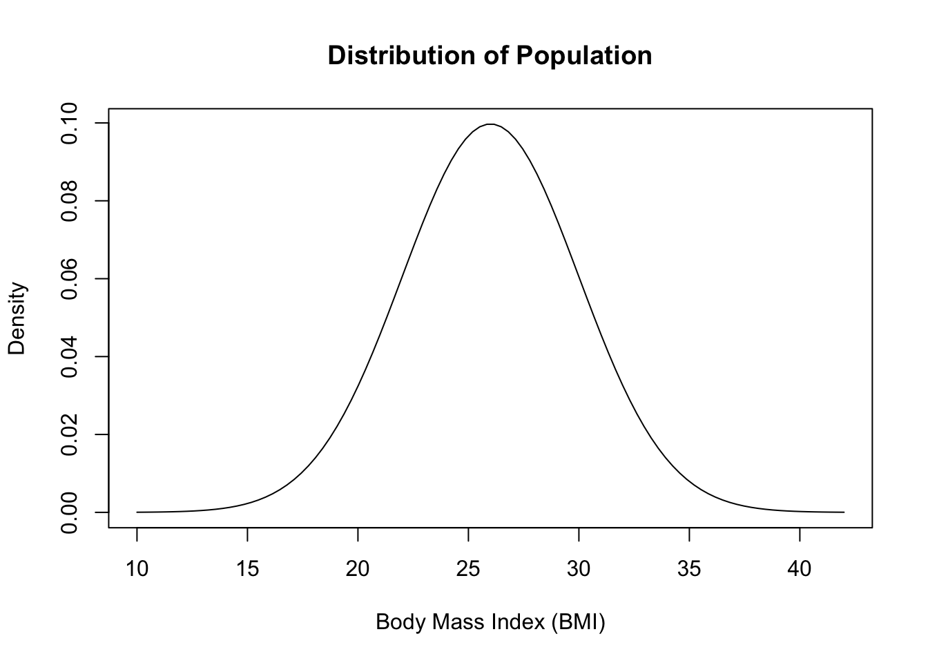
Warning
After running the code, be sure the output looks correct.
Picking One Random Sample
We can use the command rnorm(n, mean, sd) to pick a random sample of size \(n\) from a normal distribution \(N(\mu, \sigma)\).
Question 3
Replace the question mark in the code cell below to randomly select 4 individual BMI’s from the population \(X \sim N(26,4)\).
Solution to Question 3
Edit and run the code cell below.
# enter a command to randomly picks 4 values from N(26,4)
my.sample <- ??

my.sample  # print your sample to the screen
Question 4
Calculate the mean and standard deviation of your sample stored in my.sample using the code below. After computing the statistics to summarize your sample, consider the following questions:
- How do your sample statistics compare to the population parameters \(\mu = 26\) and \(\sigma =4\)?
- How do expect your sample statistics will compare to the statistics that others in class obtain from their own random samples?
# enter a command to compute the mean of my.sample

# enter a command to compute the st. dev. of my.sample
Solution to Question 4
After checking the output of the code cell above, be sure to address the two questions in the bullets above.
Sampling Distribution for BMI Means with \(n=4\)
A sample of \(n=4\) adult men are randomly selected. The mean BMI of the sample is calculated using the formula for a sample mean:
\[\bar{x} = \frac{x_1 + x_2 + x_3+x_4}{4}.\]
Then we repeat this process many, many times:
- Pick a random sample of \(n=4\) adult men from the population.
- Calculate the sample mean of the new sample.
- Repeat over and over again (for example 1,000 times).
The sampling distribution of the means is the distribution of all sample means obtained by repeatedly picking random samples each of size \(n\).
- It is important to note that each sample must have the same size, \(n\).
- The sampling distribution for the mean is the distribution of all possible random samples.
- It is extremely difficult and time intensive to write and run code that generates every possible random sample once, without any duplicates.
- In practice, we generate many (say 1,000) such random samples to approximate the sampling distribution.
A sampling distribution for the mean BMI for \(n=4\) can be constructed with the code below.
# creates an empty vector to store results
n4.bmi.bar <- numeric(1000)

# a for loop that generates 1000 random samples
# each size n=4, and calculates the sample mean.
for (i in 1:1000)
{
  n4.bmi.sample <- rnorm(4, 26, 4)  # randomly picks 4 values from N(26,4)
  n4.bmi.bar[i] <- mean(n4.bmi.sample)  # calculate sample mean
}

# plot the sampling distribution as a histogram
hist(n4.bmi.bar, xlim = c(14, 38),
     xlab = "Mean BMI of Sample",
     main = "Sampling Distribution of Mean BMI for n=4",
     xaxt='n')
axis(1, at=seq(14, 38, 4), pos=0)  # sets ticks on x-axis
abline(v = 26, col = "red", lwd = 2, lty = 2)  # draws vertical line at mu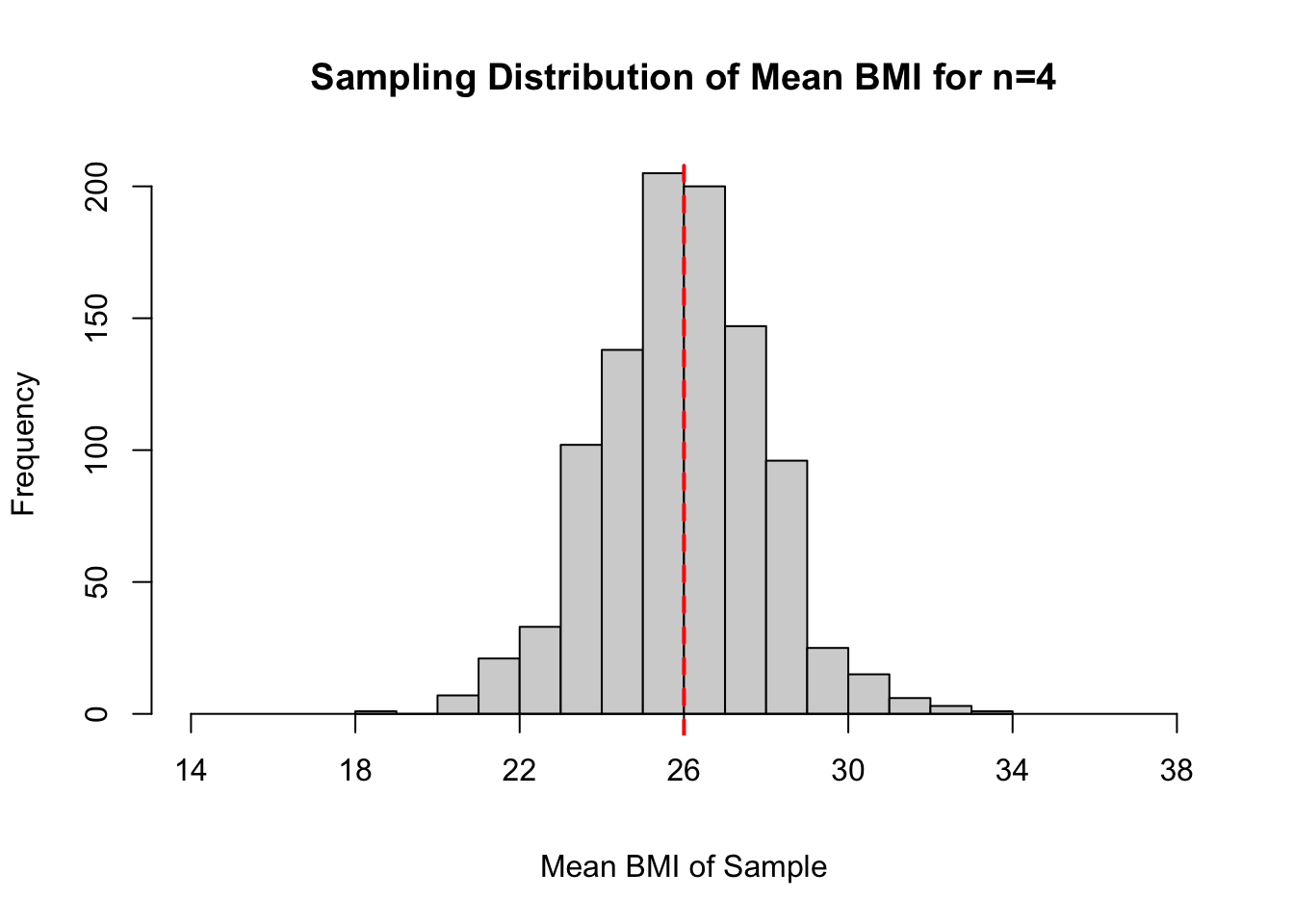
Question 5
In the code cell below, enter commands to compute the center (as measured by the mean) and spread (as measured by the standard deviation) of the sampling distribution created in the previous code cell with samples each size \(n=4\). After computing the statistics to summarize your sampling distribution, comment on how these values compare to the population parameters \(\mu=26\) and \(\sigma =4\).
Note
Sample means from the previous code cell are stored in the vector n4.bmi.bar.
# enter a command to compute the mean of the sampling dist

# enter a command to compute the st. dev. of the sampling dist
Solution to Question 5
After completing and running the code cell above, comment on how the output compares to the mean and standard deviation of the population \(X\).
Shape of the Sampling Distribution
We can use a quantile-quantile plot (also called a qq-plot) to compare the shape of our sampling distribution to the standard normal distribution \(N(0,1)\). A qq-plot is a great tool for determining how “normal” a distribution is, and we will shortly explore how to read qq-plots plots more carefully. For now we only consider the the following:
- The closer the points are to the line, the more normal the distribution.
Run the code cell below to generate a qq-plot for the sampling distribution for the mean.
qqnorm(n4.bmi.bar)
qqline(n4.bmi.bar)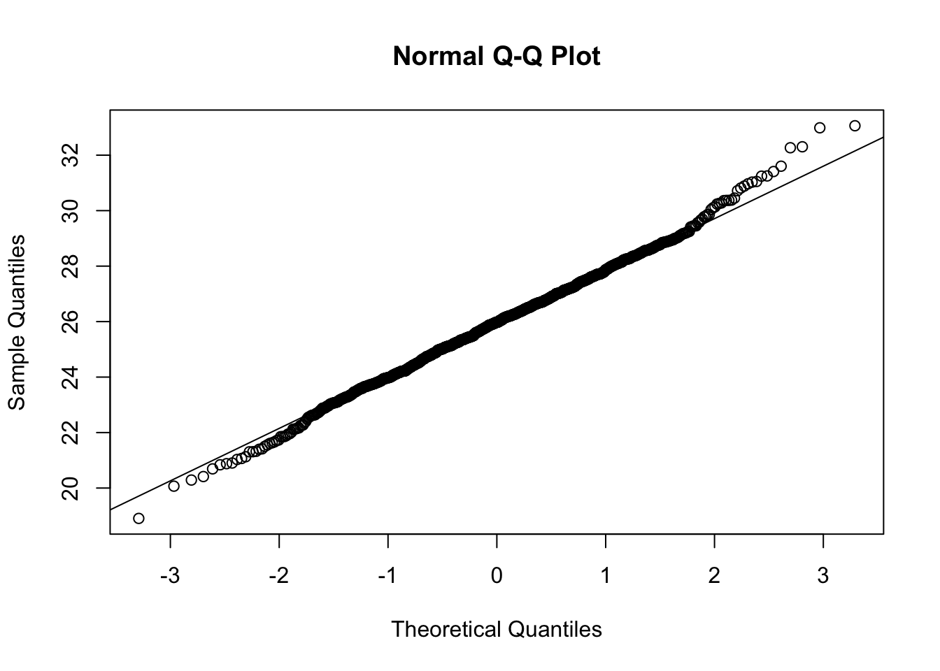
Note
The plot above seems mostly normal in the middle, but the tails are slightly deviating from the tails of a normal distribution.
Question 6
Open the app https://adamspiegler.shinyapps.io/clt_bmi/ to experiment with changing the sample size \(n\) used when constructing a sampling distribution for the mean BMI. In particular, explore the following properties of the sampling distribution for the mean BMI:
- What is the shape of the sampling distribution?
- What is the mean of the sampling distribution?
- What is the standard deviation of the sampling distribution?
- How does the population change when generating different sampling distributions?
Fill in values that describe these properties of the sampling distribution for \(n=4\), \(n=9\), \(n=16\), and \(n=81\).
Solution to Question 6
| Property | Population | \(n=4\) | \(n=9\) | \(n=16\) | \(n=81\) |
|---|---|---|---|---|---|
| Shape | Normal | ||||
| Mean | 26 | ||||
| Standard Deviation | 4 |
Sampling from a Skewed Distribution
Let \(Y\) denote all times (in minutes) that people wait before their train arrives at a certain train station. If we know the average wait time between arriving trains is \(4\) minutes, then we can use an exponential distribution to model the distribution of wait times between arriving trains. The rate parameter is \(\color{dodgerblue}{\lambda = \frac{1}{4}}\). The distribution of wait times between successive trains is therefore \(\color{dodgerblue}{Y \sim \mbox{Exp} \left( \frac{1}{4} \right)}\).
Run the code below to plot the probability density function for the train wait times, \(Y \sim \mbox{Exp} \left( \frac{1}{4} \right)\). There is nothing to edit in the code cell below, but be sure to compare the resulting plot with your answer in Question 1.
wait <- seq(0, 10, length=100)  # wait times from 0 to 10 min plotted
pdf.wait <- dexp(wait, 1/4)  # height of pdf function

plot(wait,  # wait times plotted on x-axis
     pdf.wait,  # corresponding pdf heights plotted on y-axis
     type="l",  # plot type "l" will connect points with a line
     lty=1,  # lty=1 plots solid line
     xlab="Wait Time (in minutes)",  # label on x-axis
     ylab="Density",  # label on y-axis
     main="Distribution of Population")  # main label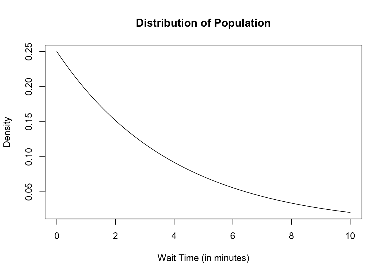
Tip
Recall that an exponential distribution \(Y\) with rate parameter \(\lambda = \frac{1}{4}\) has:
- Mean \(\mu_Y = \frac{1}{\lambda} = 4\) minutes.
- Variance \(\sigma_Y^2 = \frac{1}{\lambda^2} = 16\).
- Standard deviation \(\sigma_Y = \sqrt{16}=4\) minutes.
Question 7
Open the app https://adamspiegler.shinyapps.io/clt_wait/ to experiment with changing the sample size \(n\) used when constructing a sampling distribution of the sample mean wait time \(\overline{Y}\) between successive trains at a train station if we assume the time between successive trains is \(Y \sim \mbox{Exp} \left( \frac{1}{4} \right)\). After experimenting with the app, complete the table below to summarize your observations when sample sizes \(n=4\), \(n=9\), \(n=16\), and \(n=81\) are used to construct a sampling distribution.
Solution to Question 7
| Property | Population | \(n=4\) | \(n=9\) | \(n=16\) | \(n=81\) |
|---|---|---|---|---|---|
| Shape | Skewed Right | ||||
| Mean | 4 | ||||
| Standard Deviation | 4 |
Working with Empirical Data: Earthquake Depth
The help documentation for the data set quakes in the dplyr package provides the following summary:
“The data set give the locations of 1000 seismic events of MB \(>\) 4.0. The events occurred in a cube near Fiji since 1964.”
The data set contains the five variables listed below.
lat: Latitude of eventlong: Longitudedepth: Depth (km)mag: Richter Magnitudestations: Number of stations reporting
Run the code cell below to load the dplyr data set so we can access the quakes data set.
library(dplyr)Numerical Summary of Quakes Data
The first command will run and print the output of the summary() function that gives numerical summaries for all variables in the data set quakes. In the second and third lines of code, we use mean() and sd() functions to compute the mean and standard deviation, respectively, of the all depth values stored in quakes$depth. Run the code cells below and note the population mean and standard deviation of the earthquake depths.
# requires dplyr package loaded above
summary(quakes)
lat long depth mag
Min. :-38.59 Min. :165.7 Min. : 40.0 Min. :4.00
1st Qu.:-23.47 1st Qu.:179.6 1st Qu.: 99.0 1st Qu.:4.30
Median :-20.30 Median :181.4 Median :247.0 Median :4.60
Mean :-20.64 Mean :179.5 Mean :311.4 Mean :4.62
3rd Qu.:-17.64 3rd Qu.:183.2 3rd Qu.:543.0 3rd Qu.:4.90
Max. :-10.72 Max. :188.1 Max. :680.0 Max. :6.40
stations
Min. : 10.00
1st Qu.: 18.00
Median : 27.00
Mean : 33.42
3rd Qu.: 42.00
Max. :132.00 mean(quakes$depth)[1] 311.371sd(quakes$depth)[1] 215.5355Graphical Summary of Depth of Quakes
Before we construct a sampling distribution for the mean depth of the earthquake data in quakes, run the plot() function in the code cell below to create a density plot of the depths and get a sense of the population we will be sampling from.
plot(density(quakes$depth),  # plot density of quake depth
         xlab = "Depth (in km)",  # x-axis label
         main = "Depths of All Earthquakes in Fiji Since 1964",  # main label
         xaxt='n')  # exclude default x-axis

# set custom ticks on x-axis
axis(1, at=seq(-100, 800, 100), pos=0)
# draw vertical line at population mean
abline(v = mean(quakes$depth), col = "red", lwd = 2, lty = 2) 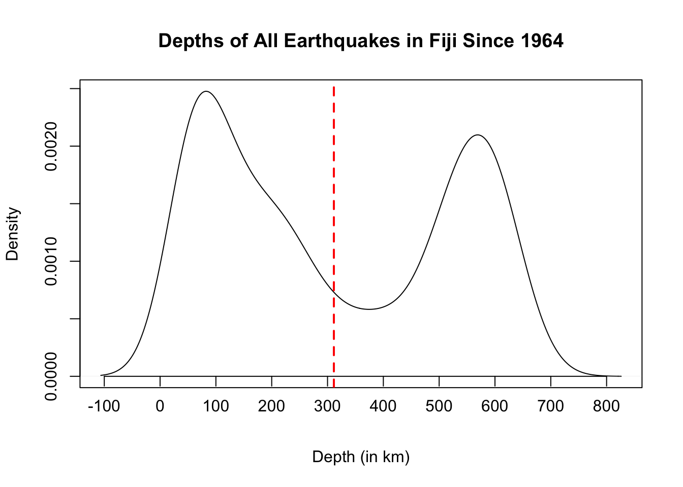
Question 8
Open the app https://adamspiegler.shinyapps.io/clt_quake/ to experiment with changing the sample size \(n\) used when constructing a sampling distribution of the sample mean earthquake depth \(\overline{Z}\) using the observed data in quakes$depth. After experimenting with the app, complete the table below to summarize your observations when sample sizes \(n=4\), \(n=9\), \(n=16\), and \(n=81\) are used to construct a sampling distribution.
Solution to Question 8
| Property | Population | \(n=4\) | \(n=9\) | \(n=16\) | \(n=81\) |
|---|---|---|---|---|---|
| Shape | Bimodal and Symmetric | ||||
| Mean | 311.37 | ||||
| Standard Deviation | 215.54 |
Notation for Population, Sample, and Sampling Distribution
Before collecting our thoughts, it will be helpful to introduce new notation to help us communicate and share observations. For each of the three contexts (BMI, train wait times, earthquake depths), we have been considering three different distributions:
- The distribution of values of the entire population.
- The distribution of values in one random sample size \(n\).
- The distribution of sample means for all random samples of size \(n\).
We can avoid some confusion by carefully using different notation when expressing the mean and standard deviation depending on whether we are summarizing a population, a sample, or a sampling distribution. When describing the mean of a distribution we use the notation:
- Population mean: \(\mu_X\)
- Sample mean: \(\bar{x}\)
- Mean of the sampling distribution for a mean: \(\mu_{\overline{X}}\)
When describing the standard deviation of a distribution we use the notation:
Population standard deviation: \(\sigma_X\)
Sample standard deviation: \(s_X\)
Spread of the sampling distribution is called the Standard Error.
The standard error measures the variability in sample statistics due to randomness.
We use the notation \(\color{mediumseagreen}{\mbox{SE}(\overline{X}) = \sigma_{\overline{X}}}\).
Organizing Observations about Sampling Distributions
Question 9
For each of the three sampling distributions we examined in Question 6, Question 7, and Question 8, summarize how the shape of the sampling distribution of the sample means changed as the size of the samples, \(n\), increased.
Solution to Question 9
Question 10
For each of the three sampling distributions we examined in Question 6, Question 7, and Question 8, summarize how the mean (center) of the sampling distribution changed as the size of the samples, \(n\), increased.
Solution to Question 10
Question 11
For each of the three sampling distributions we examined in Question 6, Question 7, and Question 8, summarize how the standard error of the sampling distribution changed as the size of the samples, \(n\), increased.
Solution to Question 11
Formal Statement of the Central Limit Theorem (for Sample Means)
Let \(X_1, X_2, \ldots , X_n\) be independent, identically distributed (iid) random variables from a population with mean \(\mu_X\) and standard deviation \(\sigma_X\), then as long as \(n\) is large enough (informally \(\mathbf{n \geq 30}\)), the sampling distribution for the mean \(\overline{X} = \frac{x_1 + x_2 + \ldots + x_n}{n}\) will:
- Be (approximately) normally distributed.
- Have mean equal to the mean of the population, \(\color{dodgerblue}{\mu_{\overline{X}}=\mu_X}\).
- Have standard error \(\color{dodgerblue}{\mbox{SE}(\overline{X}) = \sigma_{\overline{X}} = \frac{\sigma_X}{\sqrt{n}}}\).
The three statements above become more accurate as \(n\) gets larger. We summarize the results more concisely below.
\[{\large \color{dodgerblue}{\overline{X} \sim N \left( \mu_{\overline{X}} , \sigma_{\overline{X}} \right) = N \left( \mu_X , \frac{\sigma_X}{\sqrt{n}} \right)}}\]
Question 12
Using properties of the expected value of linear combinations of random variables prove the following:
\[\mu_{\overline{X}} = E \left( \overline{X} \right) = E \left( \frac{X_1 + X_2 + \ldots + X_n}{n} \right) = \mu_X.\]
Solution to Question 12
Question 13
Using properties of the variance of linear combinations of independent random variables prove the following:
\[ \sigma^2_{\overline{X}} = \mbox{Var} \left( \overline{X} \right) = \mbox{Var} \left( \frac{X_1 + X_2 + \ldots + X_n}{n} \right) = \frac{\sigma^2_X}{n}.\]
Solution to Question 13

Statistical Methods: Exploring the Uncertain by Adam Spiegler is licensed under a Creative Commons Attribution-NonCommercial-ShareAlike 4.0 International License.