We previously used sampling distributions to describe the distribution of means computed from different random samples (each the same size) picked from the same population. The standard error (standard deviation of the sampling distribution) measures how much variability to expect due to the uncertainty in the sampling process. In many situations, a mean is not a relevant or helpful statistic, and other sample statistics, such as proportions, may be more applicable to the analysis. For example:
If a jury pool of 20 people are randomly selected from a population where 42% of eligible jurors indentify their political party as Independent, what is fair representation for Independents on the jury pool?
Below are some observations to help guide our investigation in this section:
The representation could be \(8/20 = 0.40\), \(9/20 = 0.45\), but not exactly 42%.
A goal of perfect representation in all possible ways is impossible to meet.
We should choose a more obtainable goal in this situation.
The goal can vary based on factors such as the interests and backgrounds of the researchers.
The proportion of Independents varies from jury to jury.
We can consider a range of fair values.
Political affiliation is measured as a categorical variable.
In the jury example, we consider two classes: “Independent” and “Not Independent”.
There is no natural “mean” to consider in this context since the data is categorical. We can however count the number of Independents in a pool of 20 randomly selected jurors and consider what is fair proportional representation? Constructing a sampling distribution for the proportion of Independents on a randomly selected jury pool is more helpful than considering a distribution of sample means in this situation.
Sampling from a Binomial Distribution
Fair representation on a jury is one example of a situation where analyzing a distribution of sample proportions may be appropriate. Very often we encounter statistical questions that ask us to approximate or compare proportions. For example
What proportion of voters support a certain candidate running for office?
What proportion of the population follow public health recommendations?
What proportion of items manufactured are defective?
We can use a sampling distribution of proportions to help analyze statistical questions regarding proportions. In these situations:
We have a population in mind. For example, all eligible jurors.
A sample size. For example, \(n=20\) people in a jury pool.
Count the number of “successes” in each sample. How many independents, \(X\), are in the pool?
We can model the probability of \(X\) “successes” with a binomial distribution.
Calculate the corresponding sample proportion that we denote \(\color{dodgerblue}{\hat{p}}\).
\[\color{dodgerblue}{\boxed{
\hat{p} = \frac{\mbox{Number of successes}}{\mbox{Size of sample}} = \frac{X}{n}
}}.\]
Note
The \(\hat{p}\) symbol for a sample proportion is pronounced “p hat”.
A sampling distribution of proportions is a distribution of the sample proportions, \(\hat{P}\), computed from many (or all) random samples each size \(n\) picked independently from the same population (with probability \(p\) of picking a “success”).
Question 1
We randomly pick a pool of \(20\) people to fill a jury pool from a population where 42% of eligible jurors identify their political party as Independents. A jury pool is picked that has 8 out of 20 people in the jury pool say they are politically Independent
Question 1a
What is the value of \(p\)?
Solution to Question 1a
Question 1b
What is the value of \(\hat{p}\)?
Solution to Question 1b
Question 1c
Will the value of \(\hat{p}\) change when different jury pools are selected? If not, explain why not. If so, what would you expect the value of \(\hat{p}\) to be?
Solution to Question 1c
Question 1d
Will the value of \(p\) change when different jury pools are selected? If not, explain why not. If so, what would you expect the value of \(p\) to be?
Solution to Question 1d
Question 1e
Let random variable \(X\) denote the number of people in the jury pool that identify politically as Independent. What random variable can we use to model the probabilities of picking different values of \(X\)?
Solution to Question 1e
Simulating a Sampling Distribution of Proportions
Before investigating the theory, we will first walk through a statistical simulation for constructing a sampling distribution for proportions from many randomly selected samples. Hopefully we can see similarities in this process as with our initial construction of sampling distributions for means, and these connections will be useful in constructing sampling distributions with statistics. We will compare the results of the simulation with the theory we explore after.
Simulating Jury Selection with sample()
We first pick one random sample size \(n=20\) from the population \(X \sim \mbox{Binom}(20, 0.42)\). The code cell below uses the sample() function to simulate randomly selecting a pool of 20 jurors from a population where 42% of voters identify as Independents and the remaining 58% of voters do not identify as Independent.
Note 5 out of the 20 people stored in jury.pool identify their political party as Independent.
Tip
Tip: The command set.seed(937) fixes the randomization used each time the sample() command is run so the same output is generated every time.
Feel free to delete the set.seed() command to appreciate the variability in random sampling.
# set seed for randomization so results do not changeset.seed(937) jury.pool <-sample(c("Indep", "Not"), # each time we select either Indep or Notsize =20, # pick 20 people for the poolreplace =TRUE, # replace the value each time before resamplingprob =c(0.42,0.58)) # probabilities of success ("Indep") and failure ("Not")jury.pool # print results to screen
The command sum(jury.pool == "Indep") counts how many values in the vector jury.pool are equal to the string “Indep”.
Based on the output stored in jury.pool from the previous code cell, the output \(5\) is stored in x.
Thus, the sample proportion stored in p.hat is \(\hat{p} = \frac{5}{20} = 0.25\).
# out of the 20 values in jury.pool# count how many equal the string "Indep"x <-sum(jury.pool =="Indep") n <-20# jury pool is size n=20p.hat <- x / n # compute p-hat p.hat
[1] 0.25
Tip
The command mean(jury.pool == "Indep") is a more concise way to calculate a sample proportion. The mean() function will both sum the number of “Indep” in jury.pool and divide by the length of the vector jury.pool, resulting in a sample proportion.
# sample proportion with `mean()`mean(jury.pool =="Indep")
[1] 0.25
Constructing a Distribution of Sample Proportions
To construct a sampling distribution of proportions, we repeat the two steps above over and over again.
Pick a random sample of \(n=20\) using the sample() function.
Calculate \(\hat{p}\) using a logical test and either a sum() or mean() function.
The for loop in the code cell below repeats the two previous steps 10,000 times and stores each sample proportion in a vector named samp.prop. Run the code cell below to generate a possible sampling distribution for proportions.
There is nothing to edit in the code cell.
Do not worry, no output is printed to the screen since the output is being stored in samp.prop.
samp.prop <-numeric(10000) # creates an empty vector to store resultsn <-20# each random jury pool is size n=20# a for loop that generates 10,000 random samples for (i in1:10000){ temp.pool <-sample(c("Indep", "Not"), # pick jury poolsize =20, replace =TRUE, prob =c(0.42,0.58)) samp.prop[i] <-sum(temp.pool =="Indep")/n # calculate sample proportion}
The previous code cell generated many (10,000) random samples. We did not ensure that all possible samples are selected exactly once. Generating all possible random samples requires more intricate code that is time consuming to run.
For example, if the population of eligible voters is only 100 people, then there would be \(\begin{pmatrix} 100 \\ 20 \end{pmatrix} = 5.4 \times 10^{20}\) distinct jury pools that could be selected!
Tip
By relaxing the condition to generate every possible sample exactly once, we can get a very good approximation of the sampling distribution with much simpler code that is easier to read, modify, and run!
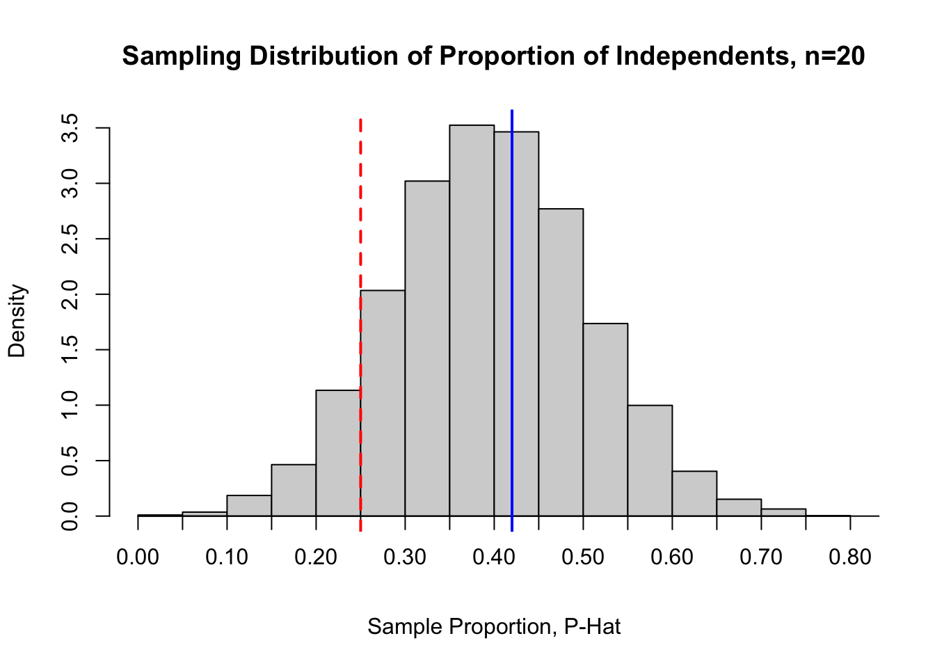
The code cell below plots a histogram of the sampling distribution of the sample proportion of Independents on a jury pool size \(n=20\). - Comments are used to help explain hist options - There is nothing to edit in the code cell.
hist(samp.prop, # plot stored sample proportionsbreaks =20, # use 20 breaksxlab ="Sample Proportion, P-Hat", # x-axis labelmain ="Sampling Distribution of Proportion of Independents, n=20", # main labelfreq =FALSE, # plot relative frequencies (density) on y-axisxaxt='n') # disable default x-axisaxis(1, at=seq(0, 1, 0.05), pos=0) # customize ticks on x-axisabline(v =0.42, col ="blue", lwd =2, lty =1) # draws vertical line at pabline(v =5/20, col ="red", lwd =2, lty =2) # draws vertical line at p-hat
Question 2
Based on the sampling distribution for the sample proportion of Independents plotted above, answer the following:
What is significant about the location of the blue vertical line plotted at \(p=0.42\) relative to the other sample proportions?
What is significant about the location of red vertical line plotted at \(\hat{p}=\frac{5}{20} = 0.25\) relative to the other sample proportions?
What is a “fair” amount of representation for Independents on a jury pool of size \(n=20\)?
Based on the values stored in samp.prop, what is the probability of randomly selecting a jury pool of \(n=20\) that has a sample proportion of Independents that is at most \(\hat{p} = 0.25\)?
Hint: Use a logical test involving samp.prop and a sum() or mean() command.
Solution to Question 2
# use samp.prop to approximate P( p-hat <= 0.25)
A Theoretical Approach
When constructing a sampling distribution for proportions, we noted that the probability of getting a certain number of “successes”, \(X\), in a sample size \(n\) can be modeled using a binomial distribution. We can make use of properties of binomial distributions to obtain a theoretical model for the sampling distribution of sample proportions. The theory gives another method for describing sampling distributions using formulas as opposed to statistical simulations that require technology.
Question 3
Let \(X \sim \mbox{Binom}(n,p)\), and consider the distribution of sample proportions \(\hat{P} = \frac{X}{n}\).
Let \(\widehat{P} = \frac{X}{n}\) denote the distribution of sample proportions. Using formulas from Question 3a and properties of expected value and variance, give formulas for \(E( \widehat{P} )\) and \(\mbox{Var}( \widehat{P} )\). Your formulas should depend on parameters \(n\) and \(p\).
Solution to Question 3b
Central Limit Theorem for Proportions
Let \(X \sim \mbox{Binom}(n,p)\) be a binomial random variable, and let \(\widehat{P} = \frac{X}{n}\) denote the distribution of sample proportions. Then if the sample size \(n\) satisfies both\(\mathbf{np \geq 10}\) and \(\mathbf{n(1-p) \geq 10}\) , the sampling distribution for \(\widehat{P}\) will:
Be approximately normally distributed.
Have mean \(\color{dodgerblue}{E(\hat{P}) = \mu_{\widehat{P}} =p}\).
Have standard error\(\color{dodgerblue}{\mbox{SE}(\widehat{P}) = \sigma_{\hat{P}} = \sqrt{\frac{p(1-p)}{n}}}\).
The standard error measures the variability in sample proportions due to the randomness in sampling.
We summarize the results of the Central Limit Theorem (CLT) for Proportions more concisely below:
\[\color{dodgerblue}{\boxed{ \widehat{P} \sim N \left( \mu_{\widehat{P}} , \sigma_{\widehat{P}} \right) = N \left( p , \sqrt{\frac{p(1-p)}{n}} \right) \qquad \mbox{ as long as both } np \geq 10 \mbox{ and } n(1-p) \geq 10.}}\]
Note
Random variable \(X\) is a discrete random variable. Using the expressions for \(E(X)\) and \(\mbox{Var}(X)\) in Question 3a, we can approximate discrete \(X \sim \mbox{Binom}(n, p)\) with continuous \(N(np, \sqrt{np(1-p)})\). The CLT for proportions essentially is stating this in terms of sample proportions \(\widehat{P}\) instead of the counts \(X\).
Question 4
Use the CLT for proportions to describe the sampling distribution for the proportion of Independents on a jury pool of \(n=20\) people. As with earlier, assume 42% of the population of eligible jurors identify their political party as Independent.
Solution to Question 4
Question 5
Based on your answer in Question 4, what is the probability of randomly picking a pool of 20 jurors that consists of at most 25% that identify politically as Independent.
Hint: Use the pnorm() function to help!
Solution to Question 5
# use CLT and pnorm()
Question 6
In Question 2 and Question 5 we use two different methods to calculate \(P( \hat{P} \leq 0.25)\), the probability of picking a jury pool of 20 people that has at most 25% that identify politically as Independent:
Question 2 uses a simulation to approximate the sampling distribution for the proportion of Independent.
Question 5 uses the CLT to theoretically model the sampling distribution.
Compare each of the values you obtained for \(P( \hat{P} \leq 0.25)\) in Question 2 and Question 5. Which do you believe is more accurate and why?
Solution to Question 6
How Large Does \(n\) Need to Be?
In the jury pool example, we have \(n=20\), \(p=0.42\), and thus \(np = 8.4 < 10\). Our sample is not seemingly large enough for the CLT according to the conditions stated for proportions above. However, the \(np \geq 10\) and \(n(1-p) \leq 10\) conditions are more like general guidelines. We can check how consistent the results of the sampling distribution simulation (results of for loop stored in samp.prop) are with the CLT:
The code cell below checks how closely our simulation matches the result \(\mu_{\widehat{P}} = E(\widehat{P}) = p=0.42\).
mean(samp.prop)
[1] 0.42013
The code cell below checks how closely our simulation matches the result \(\sigma_{\widehat{P}} = \mbox{SE}(\widehat{P}) = \sqrt{\frac{p(1-p)}{n}}=0.1104\).
sd(samp.prop)
[1] 0.1101817
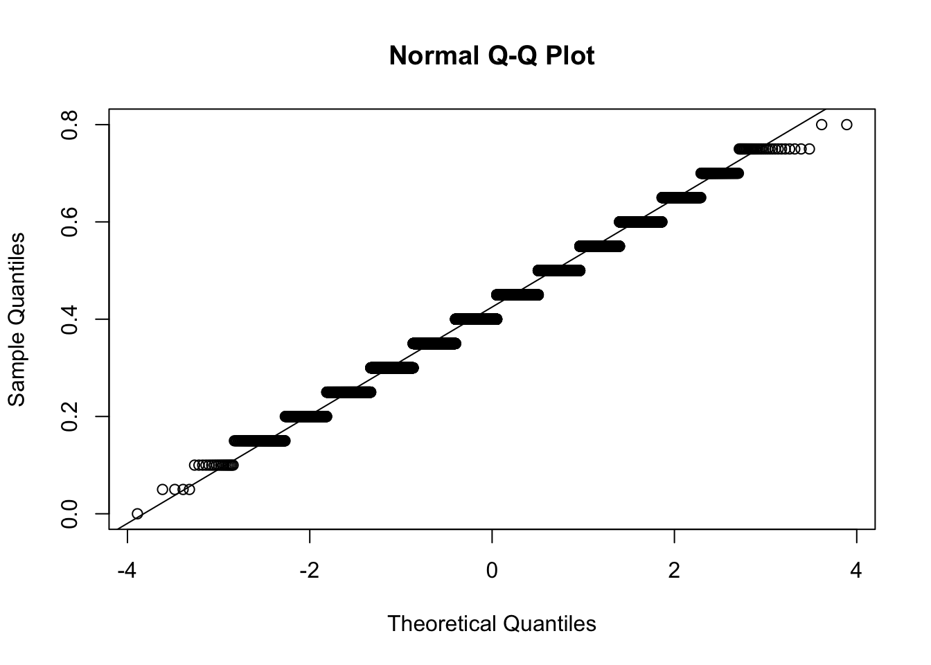
The code cell below uses a quantile-quantile plot to compare the distribution of sample proportions from our simulation to the standard normal distribution.
The sampling distribution distribution is fairly close to the line in the qq-plot!
qqnorm(samp.prop)qqline(samp.prop)
We see all three results regarding the center, spread, and shape of the sampling distribution of sample proportions are reasonably accurate in the jury pool example even though the conditions of the “rule” are not quite satisfied.
In the statement of the Central Limit Theorem for proportions, we state the theorem applies as long as both \(np \geq 10\) and \(n(1-p) \geq 10\).
The \(np \geq 10\) and \(n(1-p) \geq 10\) criterion is not a set rule that must be satisfied.
If the conditions are met, then a normal distribution is a good approximation.
If the conditions are not met, then a normal distribution may still be a good approximation. Compare distributions!
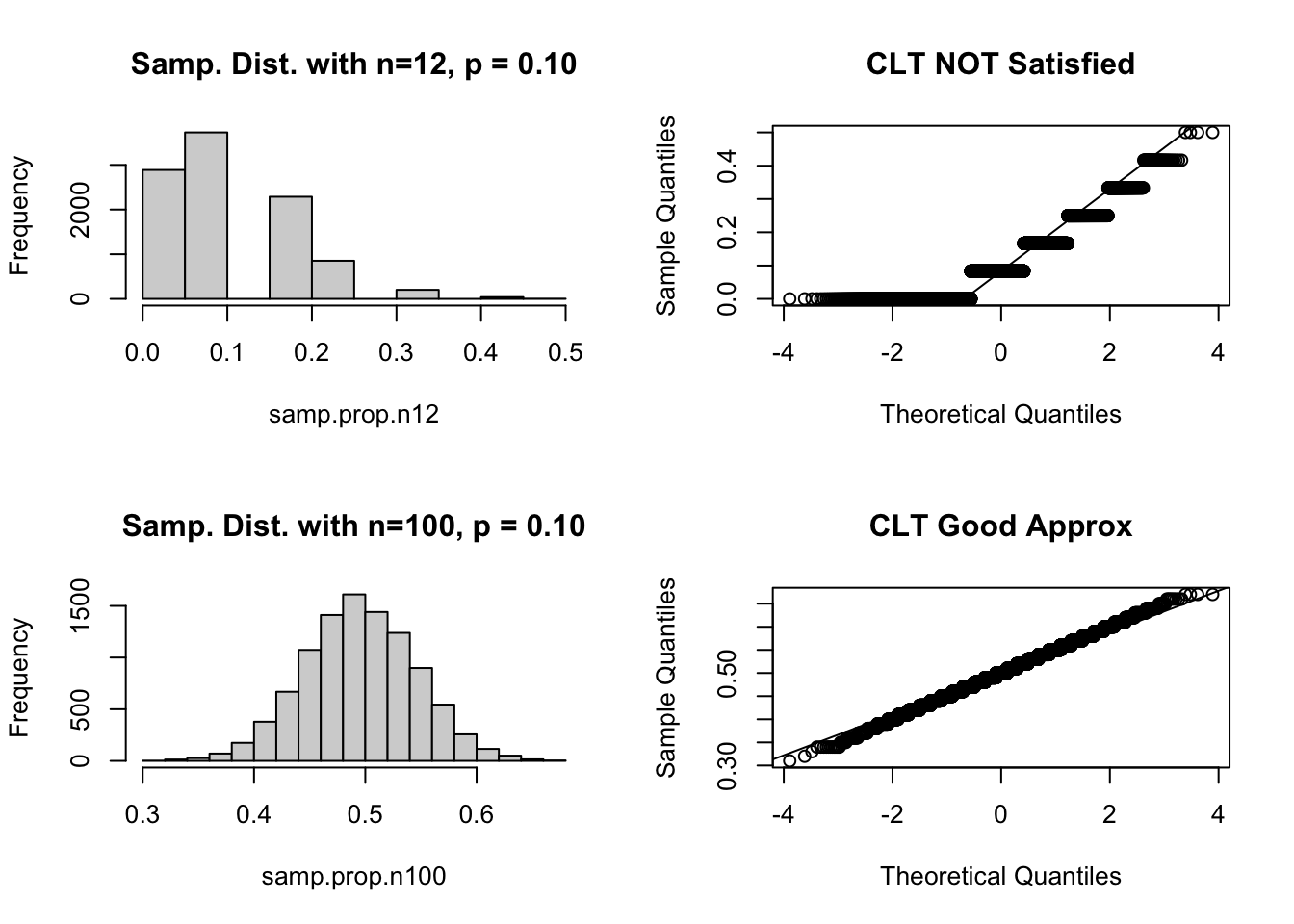
Whether a normal distribution is a good approximation depends on both the sample size \(n\) and the proportion \(p\).
The larger \(n\) is, the better the more normal (\(p\) closer to 1 or 0 can be okay).
The closer \(p\) is to \(0.5\), the more normal (smaller \(n\) can be okay).
It is always a good to compare/check numerical and theoretical results to be sure!
If our sample is not large enough (either \(np < 10\) or \(n(1-p) < 10\)) then sampling distribution of the sample proportions:
Will still satisfy \(E(\widehat{P}) = p\).
Will still have standard error \(\mbox{SE}( \widehat{P}) = \sqrt{\frac{p(1-p)}{n}}\).
But may NOT be normally distributed.
Comparing Binomial and Normal Distributions
When constructing a sampling distribution of sample proportions, we approximate the distribution of sample proportions with a continuous distribution, namely a normal distribution. However, the possible sample proportions we can get from a sample size \(n\) are not continuous. The possible sample proportions are a discrete set.
In the jury example, we have \(n=20\) and \(X = \left\{ 0, 1, \ldots , 19, 20 \right\}\).
Thus, the possible sample proportions are \(\hat{p} = \left\{ 0, 0.05, 0.10, \ldots , 0.95, 1 \right\}\).
However, in Question 5 we approximate \(\hat{P} \sim N( 0.42, 0.1104)\) with a continuous, normal distribution.
Note: We could equivalently use \(N \big( 0.42, \sqrt{(20)(0.42)(0.58) \big)}\) to approximate \(X \sim (20, 0.42)\) and have the same issue.
We can see this discrepancy between discrete data and continuous approximation in the step-like pattern in the previous qq-plots.
Warning
Since CLT for Proportions uses a continuous (normal) distribution to approximate a discrete (binomial) distribution, any results obtained using CLT will be approximations, not exact.
Question 7
Consider the same jury pool example where we randomly select a jury from a population where 42% of eligible jurors identify their political party as Independent. Let \(X\) denote the number of Independents on jury pool size \(n=20\). Use a binomial distribution to calculate the \(P(X \leq 5)\), the probability that at most 5 out of 20 identify politically as Independents.
Solution to Question 7
# use a binomial function to answer question 7
Comparing Binomial Distribution to Approximation from the CLT
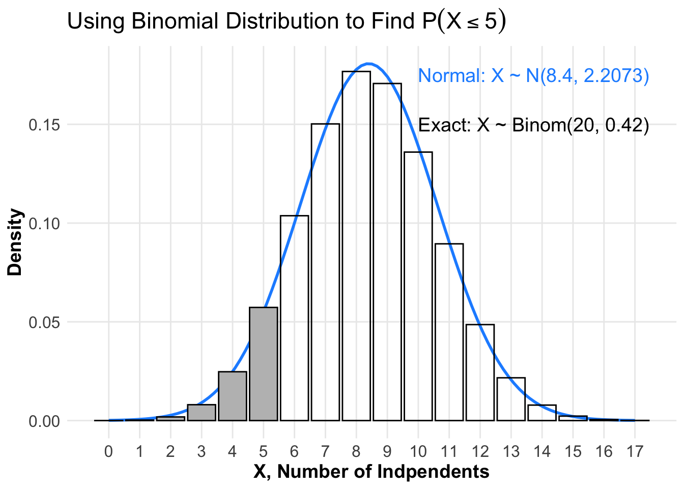
In the jury pool example, the discrete binomial distribution \(X \sim \mbox{Binom}(20, 0.42)\) is used to identify the probability of getting exactly \(X\) Independents in a jury of \(n=20\). From the CLT for proportions, we have \(\color{dodgerblue}{\widehat{P} \sim N \left(p , \sqrt{\frac{p(1-p)}{n}} \right) = N(0.42, 0.1104)}\), which is also equivalent to the approximation \(\color{dodgerblue}{X \sim N \left( np , \sqrt{np(1-p)} \right) = N(8.4, 2.2073)}\). The figure below illustrates and compares how we can use different distributions to estimate the same probabilities.
The precise, binomial distribution \(X \sim \mbox{Binom}(20, 0.42)\) is plotted as a histogram.
In Question 7, we used \(X \sim \mbox{Binom}(20, 0.42)\) to calculate \(P(X \leq 5) = 0.0922\).
The normal approximation for \(X\) is \(N \big( np, \sqrt{np(1-p)} \big) = N (8.4, 2.2073)\) and plotted in blue.
Warning: Using `size` aesthetic for lines was deprecated in ggplot2 3.4.0.
ℹ Please use `linewidth` instead.
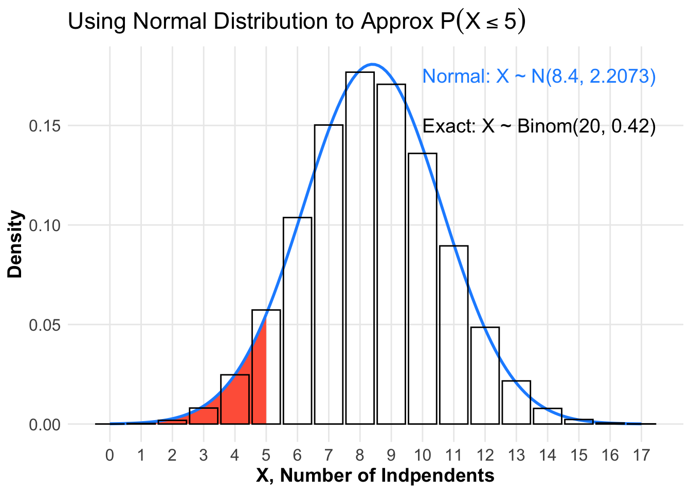
In Question 5, we used the CLT for proportions to approximate \(P(\widehat{P} \leq 0.25) \approx P( X \leq 5) \approx 0.0617\).
The region corresponding to the approximation \(\color{tomato}{P( X \leq 5) \approx 0.0617}\) is shaded in red.
This is the area to right of \(X=5\) below graph of the normal approximation for \(X\) given by \(N (8.4, 2.2073)\).
Comparing areas in the figure below, we see the area shaded in red is smaller than the actual area of the rectangles over \(X=0,1,2,3,4, \mbox{ and } 5\).
Using a normal distribution to approximate areas below a binomial distribution will result in an underestimate.
Using a normal distribution to approximate the binomial distribution, we have \(\color{dodgerblue}{\widehat{P} \sim N(0.42, 0.1104)}\).
In Question 5, we used the CLT for proportions to calculate \(\color{dodgerblue}{P(\widehat{P} \leq 0.25) = P( X \leq 5) \approx 0.0617}\).
Comparing areas in the figure below, we see the area shaded in red is smaller than the actual area of the rectangles over \(X=0,1,2,3,4, \mbox{ and } 5\).
Using a normal distribution to approximate \(P(\widehat{P} \leq 0.25)\) results in an underestimate.
Continuity Correction for Discrete Random Variables
In the previous plot, we note using a normal distribution to approximate a binomial distribution results in an underestimate since we miss capturing some of the rectangular area below the binomial distribution. We can improve the estimates we obtain using a normal distribution by including some additional area using a continuity correction as follows.
To more accurately calculate \(P( a \leq X \leq b)\) where \(a < b\) are integers, then we apply the following correction:
Shift the lower cutoff \(X=a\) half a unit further to the left, to \(X = a-0.5\).
Shift the upper cutoff \(X=b\) half a unit further to the right, to \(X = b+0.5\).
If we use the CLT for proportions to approximate the distribution of sample proportions as \(\widehat{P} \sim N \left( p, \sqrt{\frac{p(1-p)}{n}} \right)\), then using proportions, the two corrected cutoffs will be:
Corrected lower sample proportion is \(\hat{p}^*_{\rm lower} = \dfrac{a-0.5}{n}\).
Corrected upper sample proportion is \(\hat{p}^*_{\rm upper} = \dfrac{b+0.5}{n}\).
Applying a continuity correction to sample proportions, we have an improved estimate:
\[\color{dodgerblue}{P( a \leq X \leq b) \approx P \left( \frac{a-0.5}{n} < \widehat{P} < \frac{b+0.5}{n} \right)}.\]
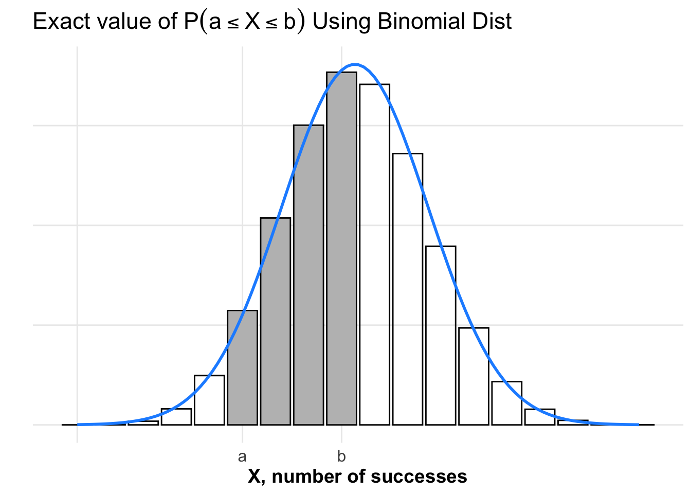
Plot of Exact Area Under Binomial Distribution
We can use the binomial distribution \(X \sim \mbox{Binom}(n, p)\) to compute the exact value of \(P(a \leq X \leq b)\). We add up the areas of each of the shaded rectangles.
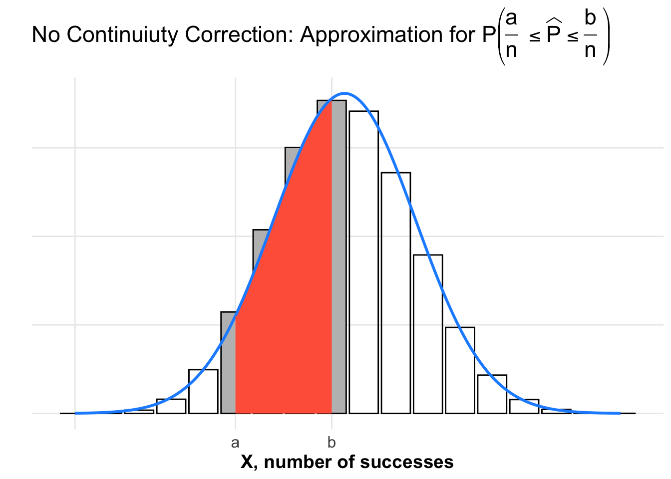
Plot of Normal Approximation Without a Continuity Correction
If we use the CLT for proportions we get \(\widehat{P} \sim N \left( p, \sqrt{\frac{p(1-p)}{n}} \right)\). Using the CLT for proportions without applying a continuity correction, we get an underestimate \(P \left( \frac{a}{n} \leq \widehat{P} \leq \frac{b}{n} \right) \approx\) that is shaded in red below. Notice there is gray shaded area under the binomial distribution that is missing from the shaded region under the normal distribution.
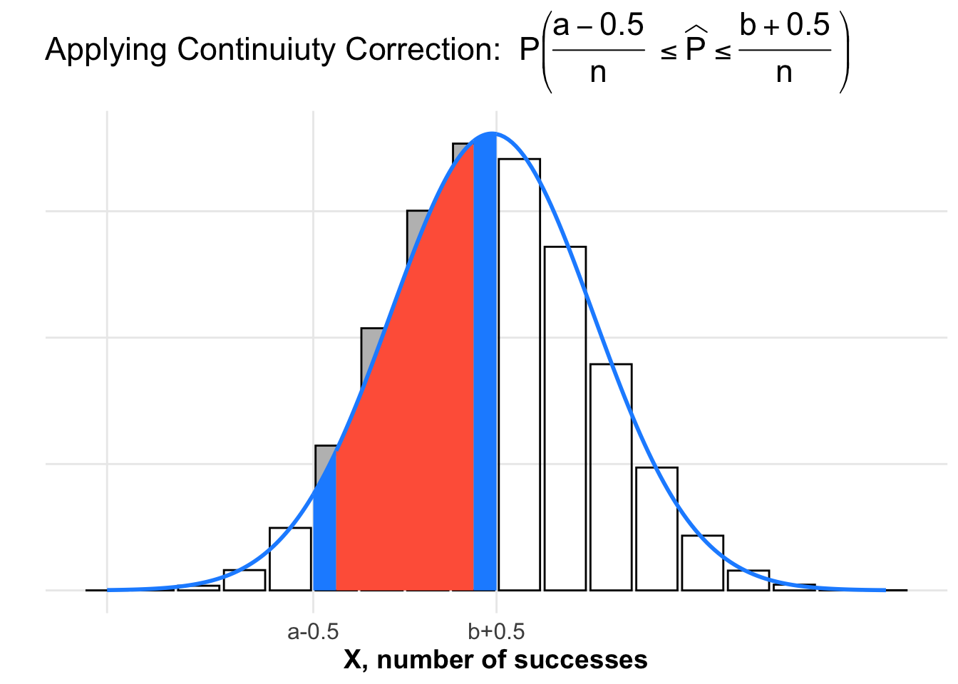
Plot of Normal Approximation With a Continuity Correction
Using the CLT for proportions along with a continuity correction, we get an improved estimate \(P \left( \frac{a-0.5}{n} \leq \widehat{P} \leq \frac{b+0.5}{n} \right)\) which is the red region plus the additional area in the two blue strips. The sum of the red and blue areas under the normal distribution is a much better approximation for the exact area under the binomial distribution.
There is a little extra area beneath the normal curve that is not included in any of the rectangular bars under the binomial distribution.
The extra area under the normal distribution approximately balances out the remaining gray rectangular areas missed above the normal distribution.
Question 8
Use the CLT for proportions along with a continuity correction to approximate the probability of randomly selecting a jury pool of \(n=20\) people that has at most 5 people that identify politically as Independent. Assume that 42% of all eligible jurors identify their political party as Independent.
Note: Although our sample size does not technically satisfy the conditions for the CLT for proportions, we verified the results hold in this example, so we may go ahead and use the CLT.
Hint: There is no correction needed for a the lower cutoff since there is no lower cutoff. You only need to apply the correction to get a new upper cutoff.
Solution to Question 8
Question 9
Census Bureau data for 2017 shows nearly half (48 percent) of residents in the United States’ five largest cities now speak a language other than English at home1. If a sample of 150 people is selected at random from the five largest cities in the US, what is the probability that between 44% and 48% of people in the sample speak a language other than English at home?
Question 9a
Is \(n\) large enough to use the CLT? Explain why or why not?
Solution to Question 9a
Question 9b
Using the CLT for a proportion, find the \(z\)-scores of the proportions \(0.44\) and \(0.48\).
Solution to Question 9b
Question 9c
Using the \(z\)-scores from Question 9b, what is the probability that between 44% and 48% (out of the random sample of 150 people) speak a language other than English at home?
Solution to Question 9c
Question 9d
Using the CLT for a proportion along with a continuity correction, give updated \(z\)-scores after applying a continuity correction to both endpoints of the interval.
Solution to Question 9d
Question 9e
Using the \(z\)-scores obtained from the continuity correction in Question 9d, what is the probability that between 44% and 48% (out of the random sample of 150 people) speak a language other than English at home?
Solution to Question 9e
Question 10
In Question 9 we calculated \(P\left( 0.44 \leq \widehat{P} \leq 0.48 \right)\) using a normal distribution (using the CLT for proportions). We could equivalently rewrite this probability in terms of the discrete random variable \(X \sim \mbox{Binom}(150,0.48)\) as \(P( 66 \leq X \leq 72\)).
Question 10a
Using a binomial distribution, calculate the exact value of \(P( 66 \leq X \leq 72\)).
Solution to Question 10a
# use binomial functions in R to solve 10a
Question 10b
Compare approximations from Question 9c and Question 9e with the exact calculation in Question 10a. Comment on whether or not the continuity correction improved the approximation or not.