2.5: Common Continuous Distributions
![]()
As we did with discrete random variables, in this section we will take a look at several of the most common and useful distributions when working with continuous random variables.
Normal Distributions
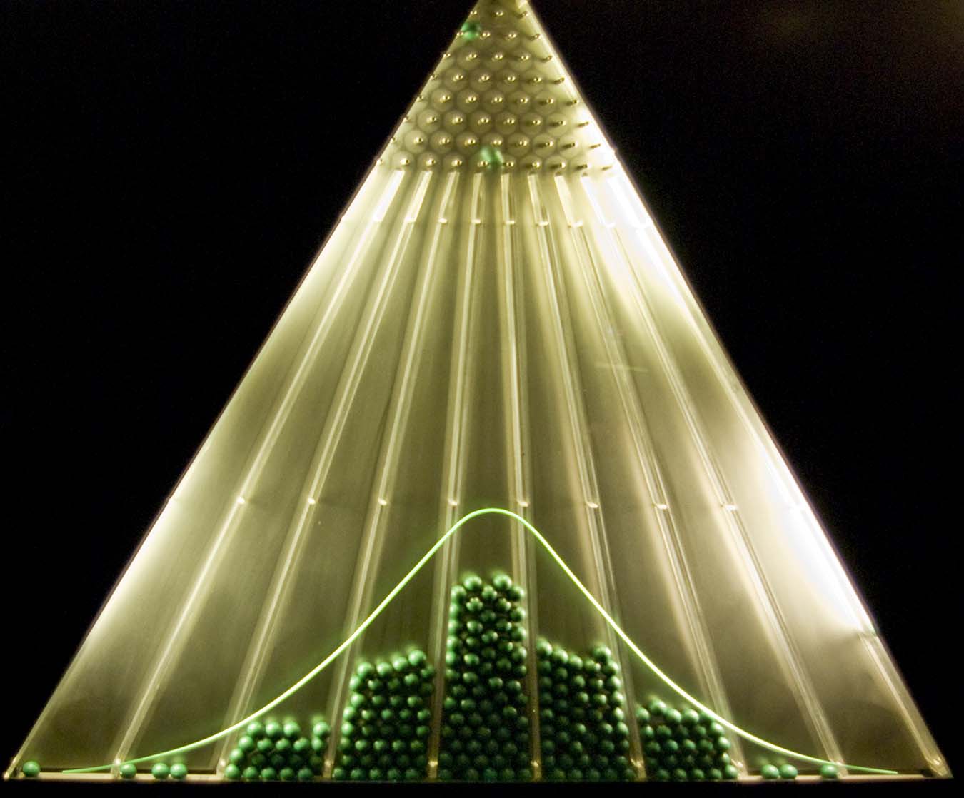
There are many situations where data tends to be distributed symmetrically around a central value with no bias to the left or right such as the location of beads on a Galton board or heights of people. For example, if we randomly select an adult from the population:
- A person is most likely to be about average height.
- Otherwise, the person selected is equally likely to be either shorter or taller than average.
- The person is very unlikely to have an extreme height (tall or short). The more extreme, the less likely.
- Therefore the distribution of heights is approximately symmetric and bell shaped.
Normal distributions arise in many settings: heights of people, size of items produced by machines, and most importantly in statistics, data sets resulting from many independent random events. The shape of a normal distribution is determined by two parameters:
- The mean, \(\color{dodgerblue}{\mu}\), is the center of the distribution.
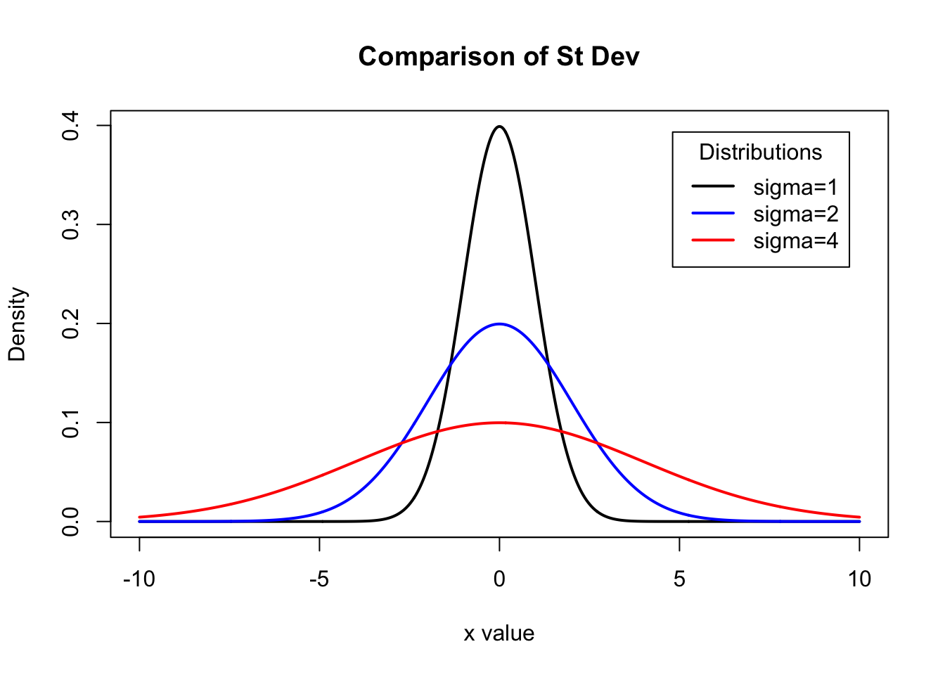
- The standard deviation \(\color{dodgerblue}{\sigma}\), tells us how wide the distribution is.
- If \(X\) is normally distributed with mean \(\mu\) and standard deviation \(\sigma\), we write \(\color{dodgerblue}{\mathbf{X \sim N(\mu, \sigma)}}\).
- The resulting distribution is symmetric and bell-shaped.
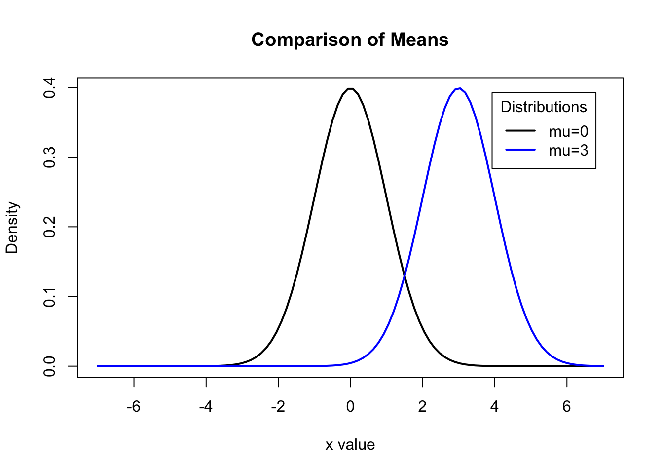
Question 1
What effect does increasing the standard deviation have on the shape of a normal distribution? What effect does increasing the mean have on the shape of a normal distribution?
Solution to Question 1
The 68%-95%-99.7% Empirical Rule
The empirical rule for normal distributions states approximately:
- 68% of all values fall within one standard deviation (both above and below) from the mean.
- 95% of all values fall within two standard deviations of the mean.
- 99.7% of all values fall within three standard deviations of the mean.

Caution
This rule does not apply to all distributions. The less normal the data, the less accurate the rule becomes.
Question 2
Cholesterol is a fat-like substance present in all cells in your body. Humans require some cholesterol to properly function and remain healthy. If a person’s blood has too much cholesterol, then they are at a higher risk of developing heart disease. A blood test is used to measure cholesterol levels. Below is an excerpt from a study1 on the distribution of cholesterol levels.
Cholesterol is a growing issue because of its impact on human health. Cigarette smoking, high blood pressure, and high blood cholesterol are the most clearly established risk factors that have been identified as being strongly associated with coronary heart disease (CHD). Total serum cholesterol level (SCL) is a major risk factor for CHD which is the leading cause of death in the United States. CHD is responsible for more deaths than all forms of cancer combined.
The distribution of cholesterol levels for adults age 20 or older is approximately normally distributed with a mean of 200 mg/dL and standard deviation 40 mg/dL. Let \(X\) be the cholesterol level of a randomly selected adult age 20 or above. Thus, we have \(X \sim N(200, 40)\).
Question 2a
What proportion of adults age 20 or above have total cholesterol levels between 200 mg/dL and 240 mg/dL?
Solution to Question 2a
Question 2b
What proportion of adults age 20 or above have total cholesterol levels between 160 mg/dL and 280 mg/dL?
Solution to Question 2b
Question 2c
Individuals that have a total cholesterol level more than 240 mg/dL should be regarded as high risk for heart disease. What proportion of the adult population age 20 or above is at high risk for heart disease?
Solution to Question 2c
Question 2d
How many standard deviations from the mean is a total cholesterol level of 140 mg/dL?
Solution to Question 2d
\(z\)-Scores and the Standard Normal Distribution
The number of standard deviations a data value \(x\) is from the mean \(\mu\) is called the z-score for the value \(x\).
- We compute the signed distance of \(x\) from the mean, \(\mu\).
- Then we describe the distance in terms of standard deviations (as opposed to in units of \(x\)).
- The formula for the \(z\)-score of \(x\) is therefore
\[\color{dodgerblue}{\large z = \frac{x-\mu}{\sigma}}.\]
For example, the \(z\)-score of an adult with a total cholesterol level of 140 mg/dL is \(z=\frac{140-200}{40} = -1.5\). This means a total cholesterol level of 140 mg/dL is 1.5 standard deviations below the mean level.
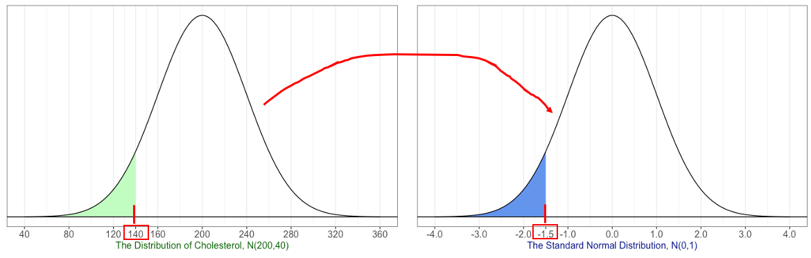
- Comparing areas in the figure above, we see that $P(X<140) = P(Z < -1.5) $.
- Thus, using either the original distribution or the distribution of \(z\)-scores gives the same result.
When we compute the \(z\)-score, we are “standardizing” the normally distributed data. We describe values of random variable \(X\) in terms of how many standard deviations each value \(x\) is from the mean \(\mu\). The resulting distribution of \(z\)-scores is called the standard normal distribution that has mean \(0\) and standard deviation \(1\).
Question 3
Body Mass Index (BMI) is often used as a measurement to determine whether a person’s weight is considered healthy. BMI is computed by dividing a person’s weight (in kilograms) by their height (in meters) squared . BMI is easy and inexpensive to measure, thus it is frequently used to screen for whether a person is malnourished, healthy, or overweight. For example, some countries have passed laws preventing companies from hiring models that are considered underweight based on BMI.
Israel became the first country ever to pass legislation banning the use of “underweight” models in local ads and publications. The new law employs an interesting tactic: Models must prove that their Body Mass Index (BMI) is higher than the World Health Organization’s indication of malnourishment (a BMI of 18.5) by producing an up-to-date medical report — no older than three months — at all shoots to be used in the Israeli market2.
Like heights and cholesterol levels, BMI distribution is approximately normal. In Israel, adult women have a mean BMI of \(26.5\) with a standard deviation \(4.5\).
Question 3a
Calculate the \(z\)-score of an adult Israeli woman with a BMI of \(18.5\).
Solution to Question 3a
Question 3b
Interpret the meaning of the value in Question 3a, and give an estimate for the proportion of adult women in Israel who are legally underweight.
Solution to Question 3b
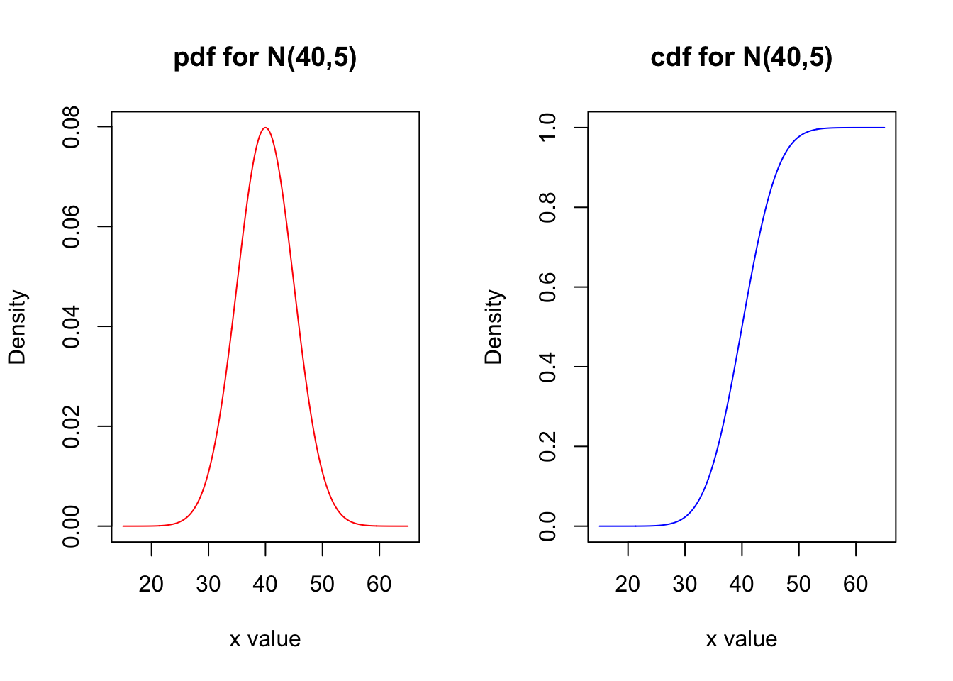
The Probability Density Function for Normal Distributions
The probability density function for a normal distribution \(X \sim N(\mu,\sigma)\) is called a Gaussian function whose formula is
\[\color{dodgerblue}{\large f(x; \mu, \sigma) = \frac{1}{\sigma\sqrt{2\pi}} e^{-\frac{1}{2} \left( \frac{x-\mu}{\sigma} \right)^2}}.\]
Note
The formula for a Gaussian depends on both irrational numbers \(\pi\) and \(e\). How surprising and cool is that!
Calculating Areas Under Normal Distributions
To find the probability that an adult woman in Israel has a BMI less than \(18.5\), we need to calculate the area to the left of \(x=18.5\) under the normal curve with formula \(f(x; 26.5, 4.5)\). We can try to evaluate
\[P(X < 18.5) = \int_{0}^{18.5} \frac{1}{4.5\sqrt{2\pi}} e^{-\frac{1}{2} \left( \frac{x-26.5}{4.5} \right)^2} \, dx\]
Important
YIKES, good luck with that! We cannot find a formula for the antiderivative of \(f(x; 26.5, 4.5)\), so we need to find other methods for calculating this area.
Using a Standard Normal Distribution Table
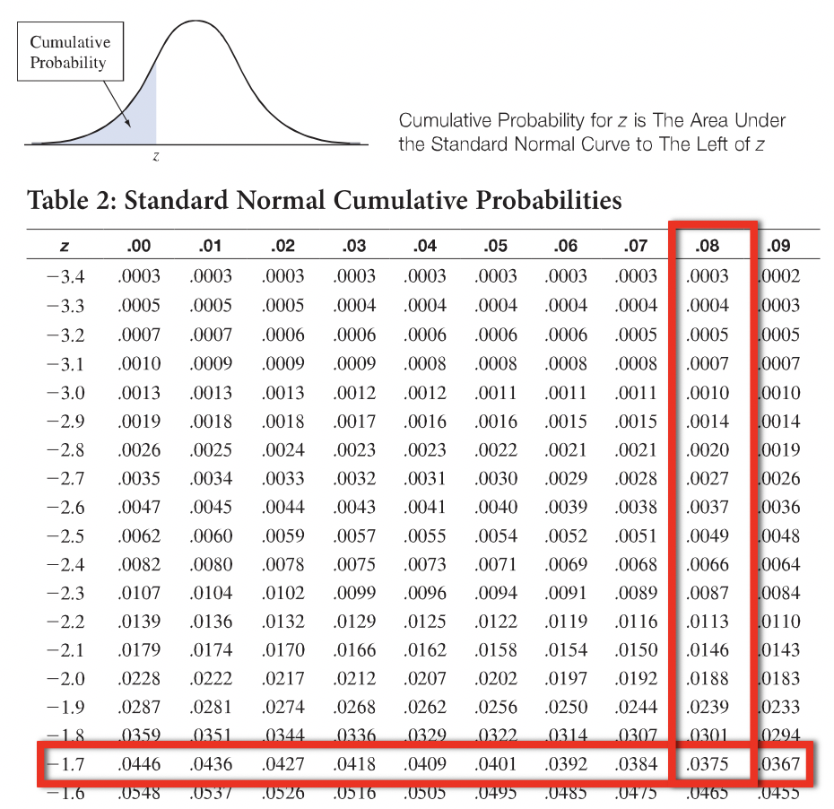
A standard normal distribution table can be used to determine the areas under the standard normal distribution, \(N(0,1)\). There are different variations of standard normal distributions. The table in the figure below gives the area under the standard normal distribution to the left of a given \(z\)-score. For example, if we want to determine what proportion of adult women in Israel have a BMI less than \(18.5\):
- Find the corresponding \(z\)-score of the BMI measurement \(x=18.5\). In Question 3a, we determined \(z \approx -1.78\).
- Look down the first column of the table and identify the row corresponding to the \(z\)-score to one decimal place of accuracy, \(z=-1.7\)
- Identify the column corresponding to the second decimal place of the \(z\)-score, \(0.08\).
- The area to the left of \(z=-1.78\) is the value located at the intersection of the row in step 2 and column in step 3.
From the figure below, we have \(P(X < 18.5) = P(Z < -1.78) \approx 0.0375\).
Using R to Compute Areas
Standard normal distribution tables were very useful prior to spread statistical software and technology. If we are working in R, we do not need to use tables to get approximations. Instead, we can use R functions to compute these areas more accurately.
Similar to binomial, geometric, and Poisson distributions, R has built in functions to perform calculations with normal distributions. In particular, the function pnorm() calculates values of the cumulative distribution function for a normal distribution:
pnorm(x, mean, sd)\(=P(X<x)\) gives the area to the left of \(x\) under \(N(\mu,\sigma)\).pnorm(x, mean, sd, lower.tail=FALSE)\(=P(X>x)\) gives the area to the right of \(x\) under \(N(\mu,\sigma)\).
Or you can find the \(z\)-score and use the standard normal distribution in R as well:
pnorm(z, 0, 1)\(=P(Z<z)\) gives the area to the left of \(x\) under \(N(0,1)\).pnorm(z, 0, 1, lower.tail=FALSE)\(=P(Z>z)\) gives the area to the right of \(x\) under \(N(0,1)\).
Warning
Do not use the function dnorm(x, mean, sd) to compute probabilities related to normal distribution since dnorm() returns the height of the probability density function. For continuous random variables, \(P(X < x)\) is the area to the left of \(x\), not the height of the function. Be sure to use pnorm(x, mean, sd) to compute \(P(X < x)\).
Question 4
Use R to compute the proportion of adult women in Israel that have a BMI below \(18.5\).
Solution to Question 4
# use code cell to help with calculation in question 4
Question 5
Intelligence quotient (IQ) scores are normally distributed. The mean IQ score is 100 points and the standard deviation is 16 points.
Question 5a
What proportion of people have an IQ score above 116?
Solution to Question 5a
Question 5b
Marilyn vos Savant has been known to have the highest recorded IQ in the world. The \(z\)-score of her test result is \(z=5.4\). What is her IQ score?
Solution to Question 5b
Question 5c
What proportion of people have an IQ score between 75 and 90?
Solution to Question 5c
Question 5d
What is the 90th percentile for IQ? In other words, find the IQ score such that 90% of the people score less than that score?
Tip
See Appendix: Normal Distributions for a summary of key formulas, graphs, shortcuts, and R functions for normal distributions.
Solution to Question 5d
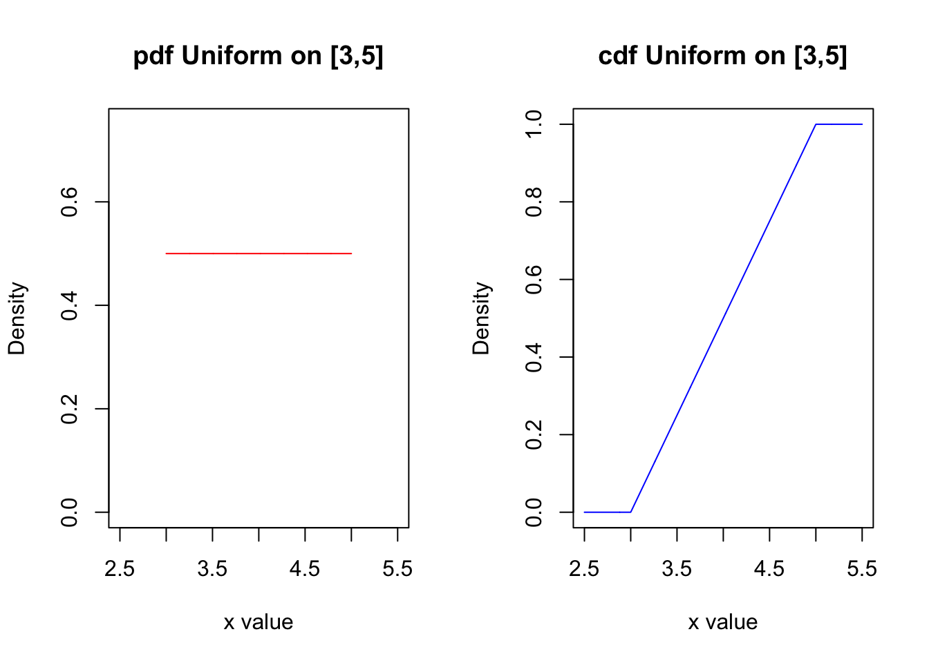
Continuous Uniform Distribution
If a continuous random variable is uniformly distributed on the interval \(\lbrack a , b \rbrack\), then the pdf is
\[f(x; a, b) = \left\{ \begin{array}{ll} \frac{1}{b-a}, & a \leq x \leq b\\ 0, & \mbox{otherwise} \end{array} \right. .\]
Question 6
Let continuous random variable \(X\) be uniformly distributed over the closed interval \(\lbrack a , b \rbrack\). Derive a formula for \(\mbox{Var}(X)\). Your answer will depend on parameters \(a\) and \(b\).
Solution to Question 6
Question 7
Let \(X\) denote the time (in minutes) spent waiting for the next light-rail to arrive at Union Station. On a separate piece of paper, sketch a possible graph for the probability distribution function of \(X\). Explain how you determined the shape of your graph.
Solution to Question 7
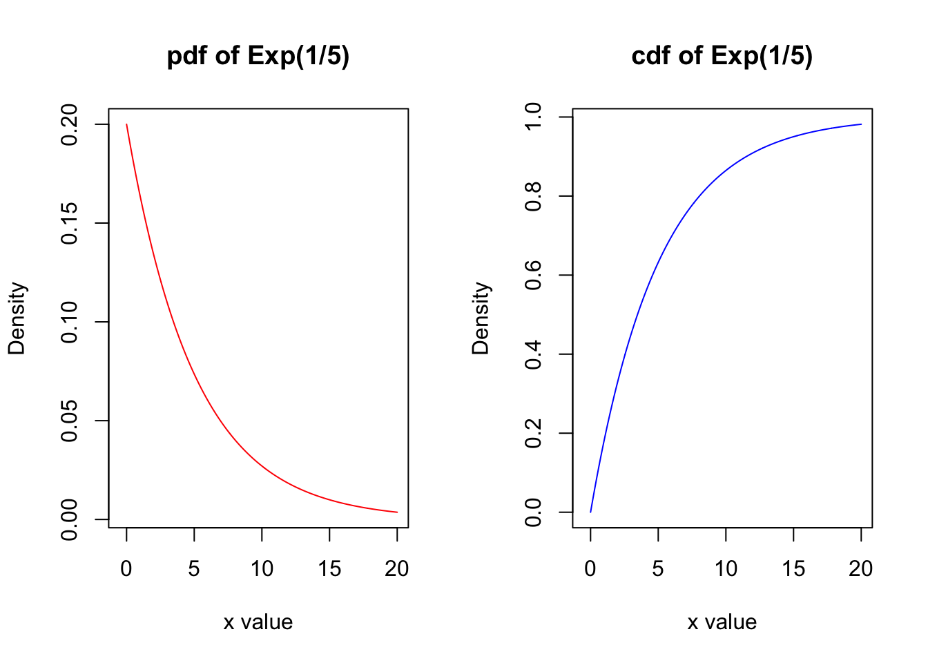
Exponential Distributions
Distributions come in all shapes in and sizes. For example:
- Uniform distributions model situations in which each outcome has an equally likely chance to occur.
- Normal distributions model distributions that are bell shaped.
Exponential distributions are often useful when considering the length of time between successive occurrences of an event.
- Most of the time, you do not need to wait very long for the next light rail.
- As the wait time \(x\) increases, it gets less and less likely that the next train has not already arrived.
- The distribution is shaped like the graph of an exponential function.
Note
See Appendix: Exponential Distributions for a summary of key formulas, graphs, shortcuts, and R functions for exponential distributions.
Question 8
At a 911 call center, calls come in at an average rate of one call every two minutes. Let \(X\) denote the time that elapses from one call to the next, and assume \(X\) has an exponential distribution.
Tip
See Appendix: Exponential Distributions for useful properties of exponential distributions.
Question 8a
Give a formula and sketch the graph of the pdf \(f\) (on a separate piece of paper).
Solution to 8a
Question 8b
Find the probability that after a call is received, it takes more than three minutes for the next call to occur. Illustrate this value on your graph in Question 8a.
Solution to 8b
Question 8c
Find a formula for the cdf, \(F\).
Solution to 8c
Question 8d
Find a formula for the inverse of the cdf, \(F^{-1}\).
Solution to 8d
Question 8e
Ninety-percent of all calls occur within how many minutes of the previous call?
Tip
Use your previous answer in Question 8d.
Solution to 8e
Question 8f
Suppose that two minutes have elapsed since the last call. Find the probability that the next call will occur within the next minute.
Tip
This is a conditional probability, so consider using Bayes’ Theorem.
Solution to 8f
Appendix: Summary of Common Continuous Random Variables
Normal Distributions
If \(X\) is normally distributed with mean \(\mu\) and standard deviation \(\sigma\), we write \(\color{dodgerblue}{X \sim N( \mu ,\sigma)}\). The formula for the probability density is called the Gaussian and is given below.
\[f(x; \mu, \sigma) = \dfrac{1}{\sigma\sqrt{2\pi}} e^{-\frac{1}{2} \left( \frac{x-\mu}{\sigma} \right)^2}\]
- The expected value is \(E(X) = \mu\).
- The variance is \(\mbox{Var} (X) = \sigma^2\).
- Use
dnorm(x, mu, sigma)to calculate \(f(x)\).- Recall for continuous distributions, \(f(x)\) gives the height of the pdf.
- Probabilities are areas under \(f(x)\) (not the heights).
- DO NOT use
dnorm()to compute probabilities.
- Use
pnorm(x, mu, sigma)to calculate \(P(X \leq x)\), the area to the left of \(X=x\).- One last warning, be sure to use
pnorm()to compute probabilities notdnorm().
- One last warning, be sure to use
- Use
rnorm(n, mu, sigma)to generate a random sample of size \(n\) from population \(X \sim N(mu, sigma)\). - Use
qnorm(q, mu, sigma)to find the qth percentile. - We have the 68%-95%-99.5% Empirical Rule.
- We can standardize the normal distribution using z-scores: \[z = \frac{x - \mu}{\sigma}\]
Continuous Uniform Distributions
\(X\) is a continuous uniform distribution when \(X\) is equally likely to equal to any value on the closed, continuous interval \(\lbrack a , b \rbrack\). If a continuous random variable is uniformly distributed on the interval \(\lbrack a , b \rbrack\), the pdf is
\[f(x; a,b) = \left\{ \begin{array}{ll} \dfrac{1}{b-a} & a \leq x \leq b\\ 0 & \mbox{otherwise} \end{array} \right. .\]
The corresponding cdf is
\[F(x) = \left\{ \begin{array}{ll} 0, & x<a \\ \frac{x-a}{b-a}, & a \leq x \leq b \\ 1, & x>b \end{array} \right. .\]
- The expected value is \(E(X) = \dfrac{a+b}{2}\)
- The variance is \(\mbox{Var}(X) = \dfrac{(b-a)^2}{12}\)
When working with uniform distributions, it is typically easier to calculate probabilities “by hand” without the need for technology. However, R does have functions to help!
- Use
dunif(x, a, b)to find the height of the pdf function, which is \(\frac{1}{b-a}\).- There is really no need to use the function since the pdf has a constant height.
- DO NOT use
dunif()to compute probabilities.
- Use
punif(x, a, b)to calculate \(P(X \leq x)=\int_a^x \frac{1}{b-a} \, dt = \frac{x-a}{b-a}\).- Probabilities can be found by computing areas of rectangles which may be easier!
- Use
runif(n, a, b)to generate a random sample of size \(n\) from population \(X \sim \mbox{Unif}(a, b)\). - Use
qunif(q, a, b)to find the qth percentile.
Exponential Distributions
Let \(X\) be the amount of time between the successive events if we know the average time between occurrences is \(\mu\). The rate parameter \(\lambda = \frac{1}{\mu}\) is the average number of times the event occurs per unit of time. Then \(X\) is exponentially distributed with rate parameter \(\lambda\), and we write \(\color{dodgerblue}{X \sim \mbox{Exp} (\lambda)}\).
The pdf for \(X \sim \mbox{Exp} (\lambda)\) is the exponential function
\[f(x; \lambda) = \lambda e^{-\lambda x} \quad \mbox{for } x >0 .\]
- The expected value is \(E(X) = \dfrac{1}{\lambda}=\mu\)
- The variance is \(\mbox{Var}(X) = \dfrac{1}{\lambda^2} = \mu^2\).
- Use
dexp(x, lambda)to find the height of the pdf function, which is \(\lambda e^{-\lambda x}\).- DO NOT use
dexp()to compute probabilities.
- DO NOT use
- Use
pexp(x, lambda)to calculate \(P(X \leq x)=\int_0^x \lambda e^{-\lambda t} \, dt\).- It never hurts to practice your integration and check with
pexp()!
- It never hurts to practice your integration and check with
- Use
rexp(n, lambda)to generate a random sample of size \(n\) from population \(X \sim \mbox{Exp}(\lambda)\). - Use
qexp(q, lambda)to find the qth percentile.
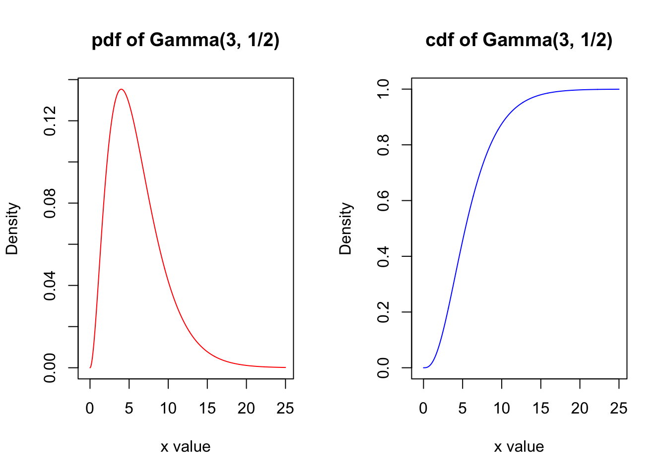
Gamma Distributions
A gamma distribution is a distribution that arises naturally in processes for which the waiting times between events are relevant. Suppose we know that \(\mu\) is the mean amount of time between successive occurrences of an event. Let \(X\) be the amount of time it takes for the event to occur \(r\) times.
- The rate parameter \(\color{dodgerblue}{\lambda = \frac{1}{\mu}}\) tells us how many times an event occurs per unit of time.
- The shape parameter \(\color{dodgerblue}{r}\) denotes the total number of occurrences we will wait to occur.
Then \(X\) will follow a gamma distribution that we denote \(\color{dodgerblue}{X \sim \mbox{Gamma} ( r, \lambda)}\). The pdf is given by
\[f(x;r, \lambda) = \frac{1}{(r-1)!} \lambda^r x^{r-1} e^{-\lambda x} \quad \mbox{for } x >0 .\]
- The expected value is \(E(X) = \dfrac{r}{\lambda}\)
- The variance is \(\mbox{Var}(X) = \dfrac{r}{\lambda^2}\).
- Use
dgamma(x, r, lambda)to find the height of the pdf function which is generally not too useful.- DO NOT use
dgamma()to compute probabilities.
- DO NOT use
- Use
pgamma(x, r, lambda)to calculate \(P(X \leq x)\). - Use
rgamma(n, r, lambda)to generate a random sample of size \(n\) from population \(X \sim \mbox{Gamma}(r, \lambda)\). - Use
qgamma(q, r, lambda)to find the qth percentile.

Statistical Methods: Exploring the Uncertain by Adam Spiegler is licensed under a Creative Commons Attribution-NonCommercial-ShareAlike 4.0 International License.