library(dplyr) # load dplyr package1.3: Exploring Quantitative Data
Click ![]() to open an interactive version of the full text section.
to open an interactive version of the full text section.
For a shorter in-class lab version of the section, part 1, click here.
For a shorter in-class lab version of the section, part 2, click here.
Additional Reading:
- See Overview of Plotting Data in R for further reading and examples about plotting in R.
- See Fundamentals of Working with Data for more information about data types and structures in R.
- The R Graph Gallery has examples of many other types of graphs.
Types of Variables
In statistics, variables are the attributes measured or collected in data. We refer to them as variables since the values or classes of attributes typically vary from observation to observation. The term variable is used differently in statistics from the notion of a variable in algebra. There are two types of variables in statistics:
- If a variable is measured or counted by a number, it is called a quantitative or numerical variable.
- Quantitative variables may be discrete (integers) or continuous (decimals).
- If a variable groups observations into different categories or rankings, it is a qualitative or categorical variable.
- The different categories of a qualitative variable are called levels or classes.
The type of statistical analysis we can do depends on whether:
- We are investigating a single variable, or looking for an association between multiple variables.
- The variable(s) are quantitative or categorical.
- The data satisfies certain assumptions.
In our work with Exploring Categorical Data, we performed an initial summary of the categorical variables in the storms data set. Today, we will investigate how to numerically and visually summarize quantitative variables.
Getting to Know Our Data
The dplyr package contains a data set from the NOAA Hurricane Best Track Data that contains data on the following attributes of tracked North Atlantic storms since 1975:
- Storm name:
name - Date and time:
year,month,day, andhour - Storm position:
latandlong - Storm classification:
status - Category of hurricane:
category(non-hurricanes areNA) - Wind speed (in knots):
wind - Pressure (in millibars):
pressure - Tropical storm force diameter (in nautical miles):
tropicalstorm_force_diameter - Hurricane force diameter (in nautical miles):
hurricane_force_diameter
Tip
See Exploring Categorical Data for a refresher on our initial exploration with the storms data frame.
Loading Required Package
In order to access the storms data frame in the dplyr package, we first load the package with the library() function.
Help Documentation for storms
The ? help operator and help() function provide access to the help manuals for R functions, data sets, and other objects. If at any point we want to learn more about data or a function used in this notebook, we can use the help operator. For example, ?typeof, ?str, ?hist, and ?boxplot will open a help tab with further details about each of function.
- Run the code cell below to access the help documentation for the
stormsdata set.
?storms # open help tabQuestion 1
List all the quantitative variables in storms. Which are being stored as integer, and which are stored as double (decimals)?
- You can edit, run and rerun the
typeof()function in the first code cell below to help identify the data types of individual variables instorms. - You can use the
str()function in the second code cell to identify the data types of all variables at once.
typeof(storms$year)[1] "double"Solution to Question 1
Question 2
What wind speeds are classified as a Category 2 hurricane?
Solution to Question 2
Question 3
What does the variable tropicalstorm_force_diameter measure? What does it mean if a storm observation has a 0 for tropicalstorm_force_diameter?
Solution to Question 3
Question 4
Enter comments in the code cell below to help describe what each command performs. Then run the str() function after running the commands to see the updated data structure of storms.
Solution to Question 4
# enter your comments after each #
storms$year <- as.integer(storms$year)  #
storms$month <- as.integer(storms$month)  #
storms$hour <- as.integer(storms$hour)  #
storms$category <- factor(storms$category)  #
# view the resulting data structure
str(storms)tibble [19,066 × 13] (S3: tbl_df/tbl/data.frame)
$ name : chr [1:19066] "Amy" "Amy" "Amy" "Amy" ...
$ year : int [1:19066] 1975 1975 1975 1975 1975 1975 1975 1975 1975 1975 ...
$ month : int [1:19066] 6 6 6 6 6 6 6 6 6 6 ...
$ day : int [1:19066] 27 27 27 27 28 28 28 28 29 29 ...
$ hour : int [1:19066] 0 6 12 18 0 6 12 18 0 6 ...
$ lat : num [1:19066] 27.5 28.5 29.5 30.5 31.5 32.4 33.3 34 34.4 34 ...
$ long : num [1:19066] -79 -79 -79 -79 -78.8 -78.7 -78 -77 -75.8 -74.8 ...
$ status : Factor w/ 9 levels "disturbance",..: 7 7 7 7 7 7 7 7 8 8 ...
$ category : Factor w/ 5 levels "1","2","3","4",..: NA NA NA NA NA NA NA NA NA NA ...
$ wind : int [1:19066] 25 25 25 25 25 25 25 30 35 40 ...
$ pressure : int [1:19066] 1013 1013 1013 1013 1012 1012 1011 1006 1004 1002 ...
$ tropicalstorm_force_diameter: int [1:19066] NA NA NA NA NA NA NA NA NA NA ...
$ hurricane_force_diameter : int [1:19066] NA NA NA NA NA NA NA NA NA NA ...Summarizing Categorical Data
When we analyze the categorical variables in storms, we use counts and proportions. In the table created by the code cell below, we see how many observations there are in each storm classification.
tbl.status <- table(storms$status) # store counts for each storm classification
tbl.status  # print table to screen
           disturbance          extratropical              hurricane
                   146                   2068                   4684
             other low subtropical depression      subtropical storm
                  1405                    151                    292
   tropical depression         tropical storm          tropical wave
                  3525                   6684                    111
The code cell below gives the proportion of storms in the data are in each storm classification.
# table of counts for each storm classification
prop.table(tbl.status)
           disturbance          extratropical              hurricane
           0.007657610            0.108465331            0.245672926
             other low subtropical depression      subtropical storm
           0.073691388            0.007919857            0.015315221
   tropical depression         tropical storm          tropical wave
           0.184884087            0.350571698            0.005821882
We used bar charts and pie charts to visualize the distribution and relations between categorical variables.
plot(storms$category,  # categorical data
     main = "Hurricanes by Category",  # main title
     xlab = "Hurricane Category",  # horizontal axis label
     ylab = "Frequency",  # vertical axis label
     col = "steelblue")  # fill color of bars)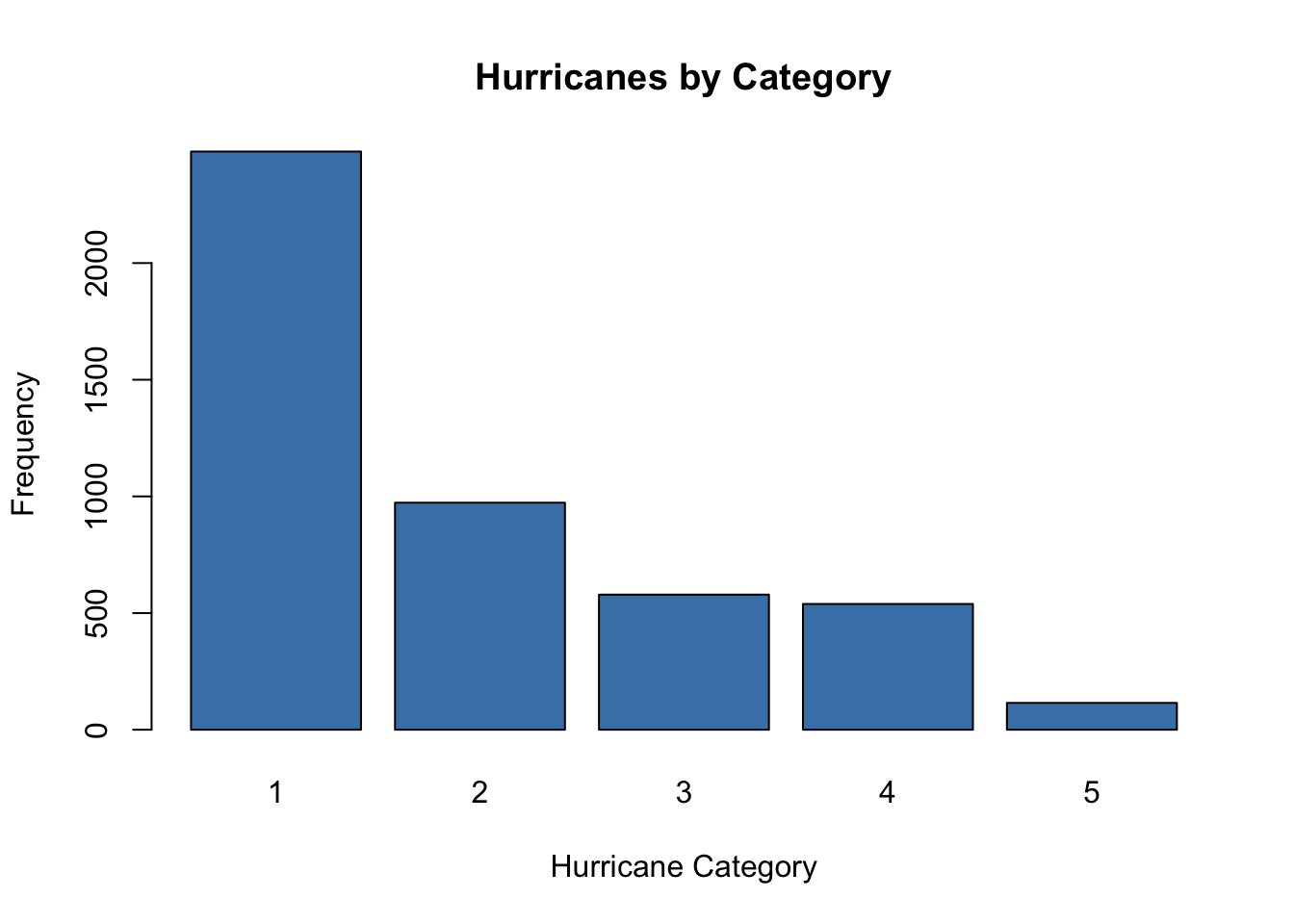
- For quantitative variables, such as wind speed (
wind), counting and proportions are not as appropriate or useful. - We get a better understanding of a quantitative variable by describing where the values are centered and the spread of the values.
- Similarly, a good visualization for a quantitative variable will help illustrate where the values are centered, how variable (spread out) the values are, and other useful properties.
Plotting Quantitative Data
Additional resources for help with plotting data:
- See Overview of Plotting Data in R for further reading and examples about plotting in R.
- The R Graph Gallery has examples of many other types of graphs.
Histograms
A histogram is special bar chart we use to display the distribution of values for a quantitative variable.
- We first group the values into different ranges of values called bins of equal width.
- This essentially converts the quantitative variable to an ordinal categorical variable with with each bin representing a different level.
- Consider the quantitative variable
wind. We can use bin ranges such as 0-10 knots, 10-20 knots, … , 160-170 knots.- Each bin range should have the same width.
- The bins do not overlap.
- The ordering of the bins is very important.
- Then we count how many values in the data are in each bin.
- A histogram is a bar chart that represents the number of values that are in each bin range.
- Values of the quantitative variable are measured on the horizontal axis.
- The height of the bars over each bin range is the number of values (or frequency) in each bin range.
- By default, the counts are right closed. For example, a wind value of 20 knots would be counted in the bin range 10-20 knots and not counted in the bin range 20-30 knots.
- A histogram should not have an spaces between consecutive bars. Empty space means no values are in that bin range.
- The R function
hist(x, [options])creates a histogram. - Run
?histfor more information about the available options for customizing a histogram, some of which are illustrated in the code cell below.
# create a histogram
hist(storms$wind,  # vector of values to plot
     breaks = 15,  # number of bin ranges to use
     xlab = "wind speed (in knots)",   # x-axis label
     xlim = c(0,200),  # sets window for x-axis
     ylab = "Frequency",  # y-axis label
     ylim = c(0,5000),  # sets window for y-axis
     main = "Distribution of Storm Wind Speed",  # main label
     col = "steelblue")  # fill color of bars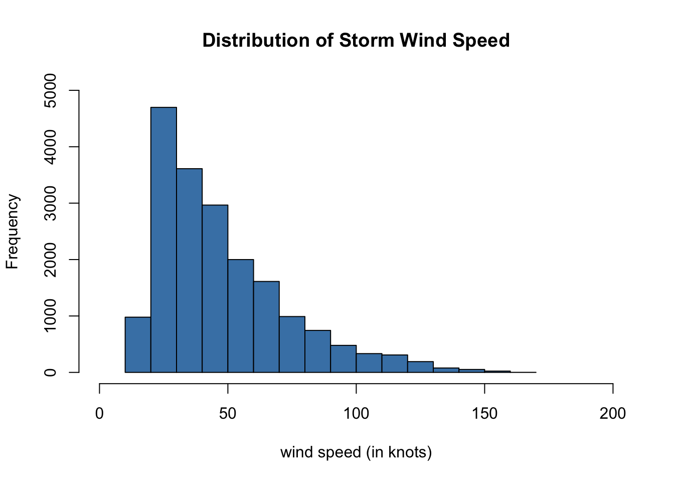
Question 5
Based on the histogram above, approximately how many storms have a wind speed less than or equal to 40 knots?
Solution to Question 5
Question 6
The code cell below can help us check our answer.
Explain what operation(s) the command in the code cell below. Running the code cell and compare the last 10 entries in the vector
le.40and the vectorstorms$windto help determine your answer.Then run and explain what the second code cell below does. Hint: R reads the logical
TRUEas the number 1 andFALSEas the number 0.How accurate was your previous answer in Question 5?
Solution to Question 6
Enter comment in first code cell.
Enter comment in second code cell.
How accurate was your answer in Question 5?
le.40 <- storms$wind <= 40  # ??

tail(storms$wind, 10)  # prints last 10 rows of wind speed vector
[1] 45 45 45 40 35 35 35 35 40 40tail(le.40, 10) # prints last 10 rows of logical vector le.40 [1] FALSE FALSE FALSE TRUE TRUE TRUE TRUE TRUE TRUE TRUE# enter comment to interpret this command
sum(le.40) # ??[1] 9288Changing the Number of Bins
A histogram can illustrate the general shape of the distribution of quantitative variable; however, the number of breaks we use can have a substantial impact.
- If we include too few bins, we do not get much detail, and we may even get a misleading picture.
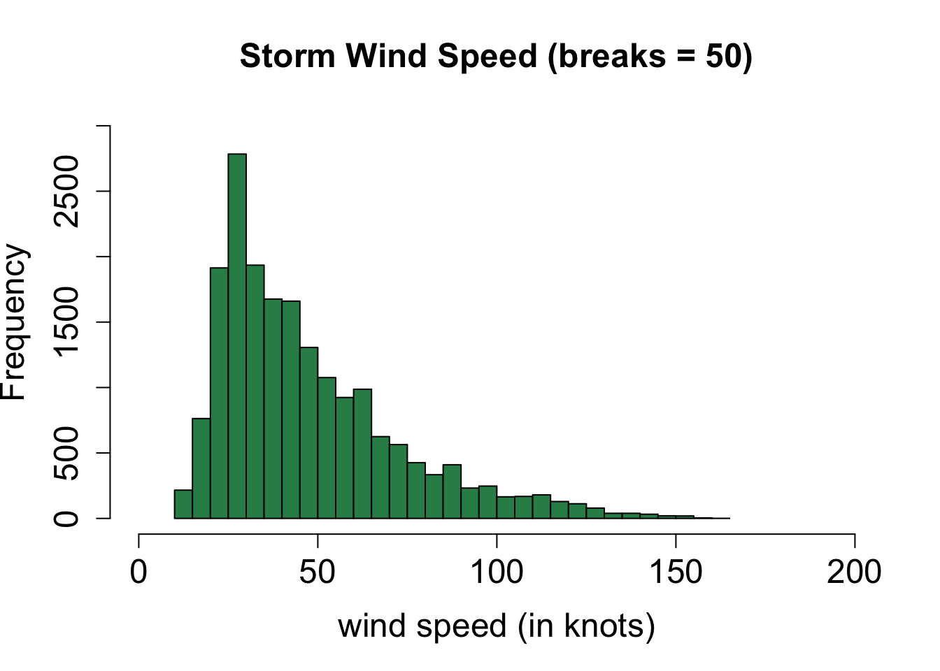
- If we include too many bins, the histogram may be difficult to read.
- The fun of interacting with data in R is we can play around and adjust the number of breaks and other options until we are satisfied.
# create a histogram
hist(storms$wind,  # vector of values to plot
     breaks = 5,  # number of bin ranges to use
     xlab = "wind speed (in knots)",   # x-axis label
     xlim = c(0,200),  # sets window for x-axis
     ylab = "Frequency",  # y-axis label
     ylim = c(0,15000),  # sets window for y-axis
     main = "Storm Wind Speed (breaks = 5)",  # main label
     cex.lab=1.5, cex.axis=1.5, cex.main=1.5,  # increase font size
     col = "steelblue")  # fill color of bars

# create a histogram
hist(storms$wind,  # vector of values to plot
     breaks = 50,  # number of bin ranges to use
     xlab = "wind speed (in knots)",   # x-axis label
     xlim = c(0,200),  # sets window for x-axis
     ylab = "Frequency",  # y-axis label
     ylim = c(0,3000),  # sets window for y-axis
     main = "Storm Wind Speed (breaks = 50)",  # main label
     cex.lab=1.5, cex.axis=1.5, cex.main=1.5,  # increase font size
     col = "seagreen")  # fill color of bars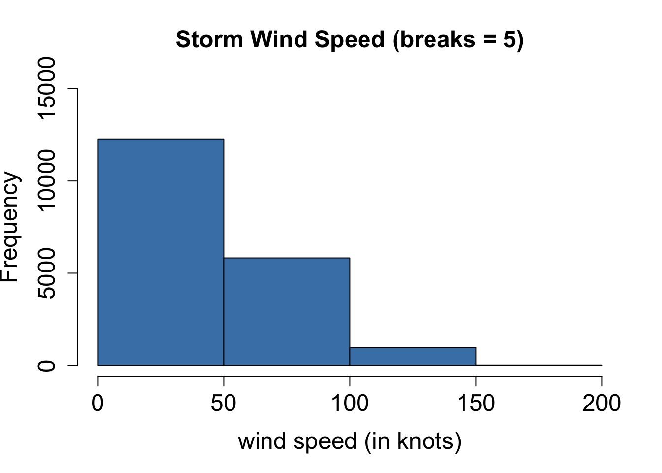
Question 7
How would you describe the shape of the distribution of wind speed in the histograms above?
Solution to Question 7
Question 8
Create a histogram to display the quantitative variable month. What does the shape of that graph tell you about the data?
Solution to Question 8
Question 9
Create a histogram to display the quantitative variable long. What does the shape of that graph tell you about the data?
Solution to Question 9
The Skewness of Data
The skewness of the data describes the direction of the tail of the data. The tail of the data indicates the direction of outliers (if any).
#par(mfrow = c(1, 3))  # Create a 1 x 3 array of plots

hist(storms$wind,
     xlab = "wind speed (in knots)",   # x-axis label
     ylab = "Frequency",  # y-axis label
     main = "Distribution of Wind Speeds",  # main title
     cex.lab=1.7, cex.axis=1.7, cex.main=1.7,  # increase font size
     col = "steelblue")  # fill color of bars

hist(storms$month,
     breaks = 12,  # number of breaks
     xlab="Month",   # x-axis label
     ylab = "Frequency",  # y-axis label
     main = "Distribution of Months",  # main title
     cex.lab=1.7, cex.axis=1.7, cex.main=1.7,  # increase font size
     col = "coral1")  # fill color of bars

hist(storms$long,
     breaks = 15,  # number of breaks
     xlab="Degrees of Longitude",   # x-axis label
     ylab = "Frequency",  # y-axis label
     main = "Distribution of Longitude",  # main title
     cex.lab=1.7, cex.axis=1.7, cex.main=1.7,  # increase font size
     col = "aquamarine4")  # fill color of bars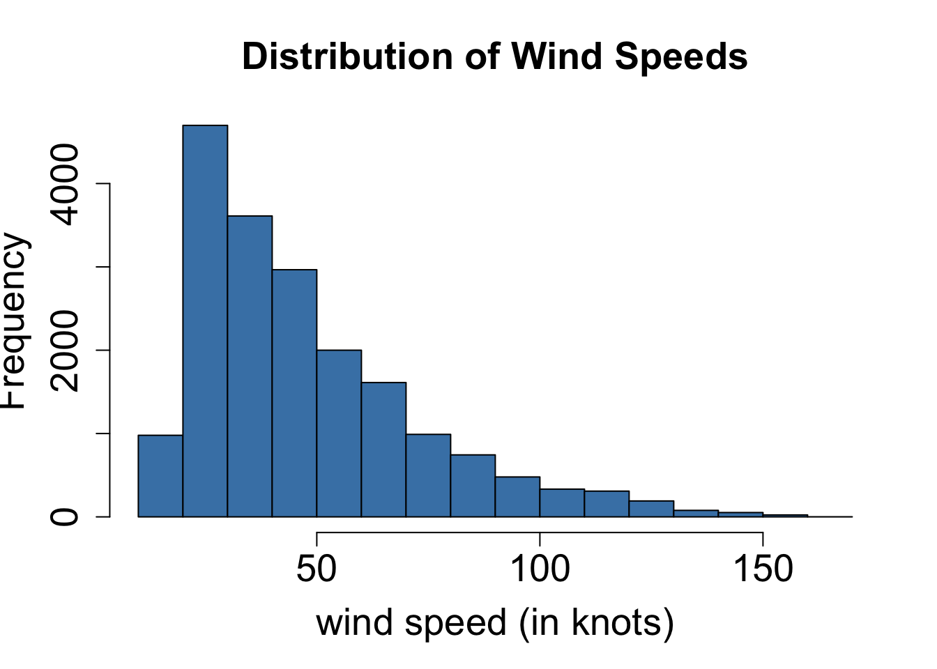
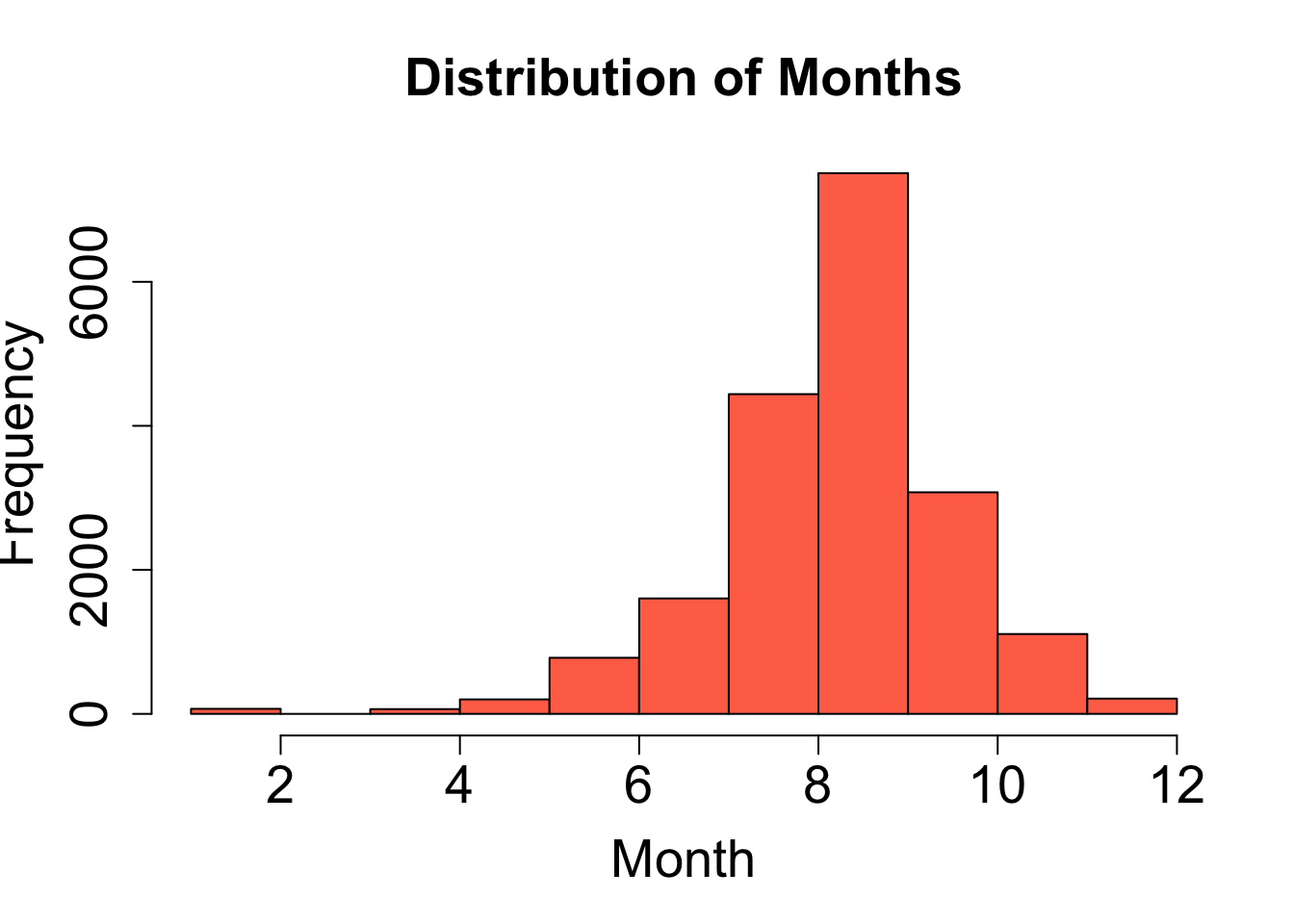
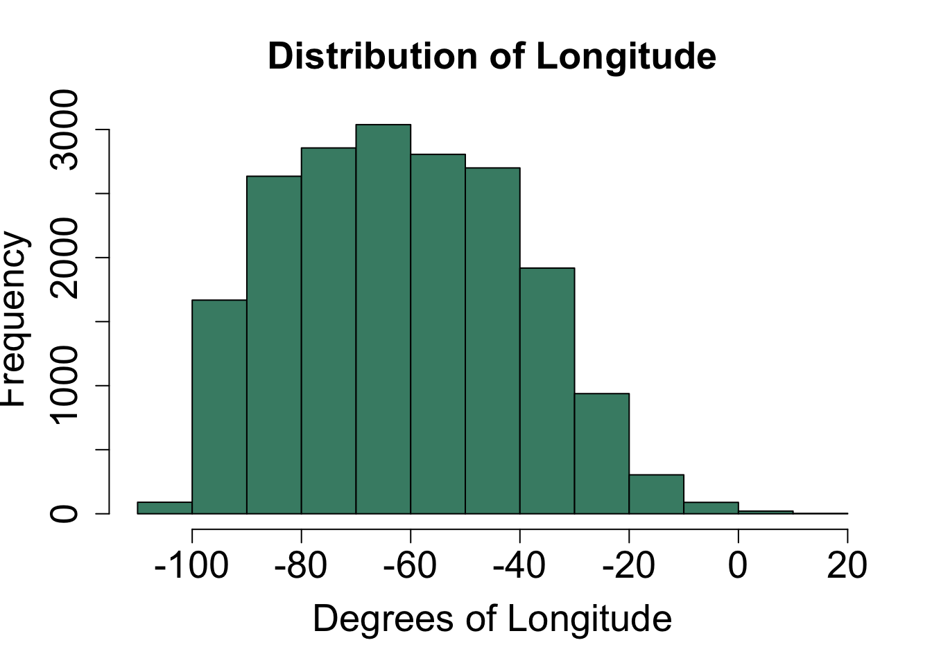
- The distribution of wind speeds is skewed right.
- The distribution of months is skewed left.
- The distribution of longitude is approximately symmetric.
Measurements of Center
Typical measurements of center are:
- The mean is the average value.
\[{\large \bar{x} = \frac{\mbox{sum of all values}}{\mbox{total number of values}} = \sum_{i=1}^{n} \frac{x_n}{n}}. \]
- We use \(\color{dodgerblue}{\mathbf{\bar{x}}}\) (pronounced x-bar) to denote a sample mean.
- We use \(\color{mediumseagreen}{\mathbf{\mu}}\) (Greek letter mu) to denote a population mean.
- In R, we use the function
mean().
- The median is the \(50^{\mbox{th}}\) percentile. This means 50% of the values in the data set are less than the median.
- In R, we use the function
median(). - If there are an odd number of values, the median is the middle value.
- If there are an even number of values, the median is the midpoint between the two middle values.
- In R, we use the function
Question 10
Compute the mean and median wind speed of the storms data. Interpret each value in practical terms. Be sure to include the units in your interpretation.
Tip
We can input the vector of wind speeds with the code storms$wind.
Solution to Question 10
Question 11
Why do you think the mean wind speed is greater than the median wind speed?
Solution to Question 11
Relation of Shape to Measurements of Center
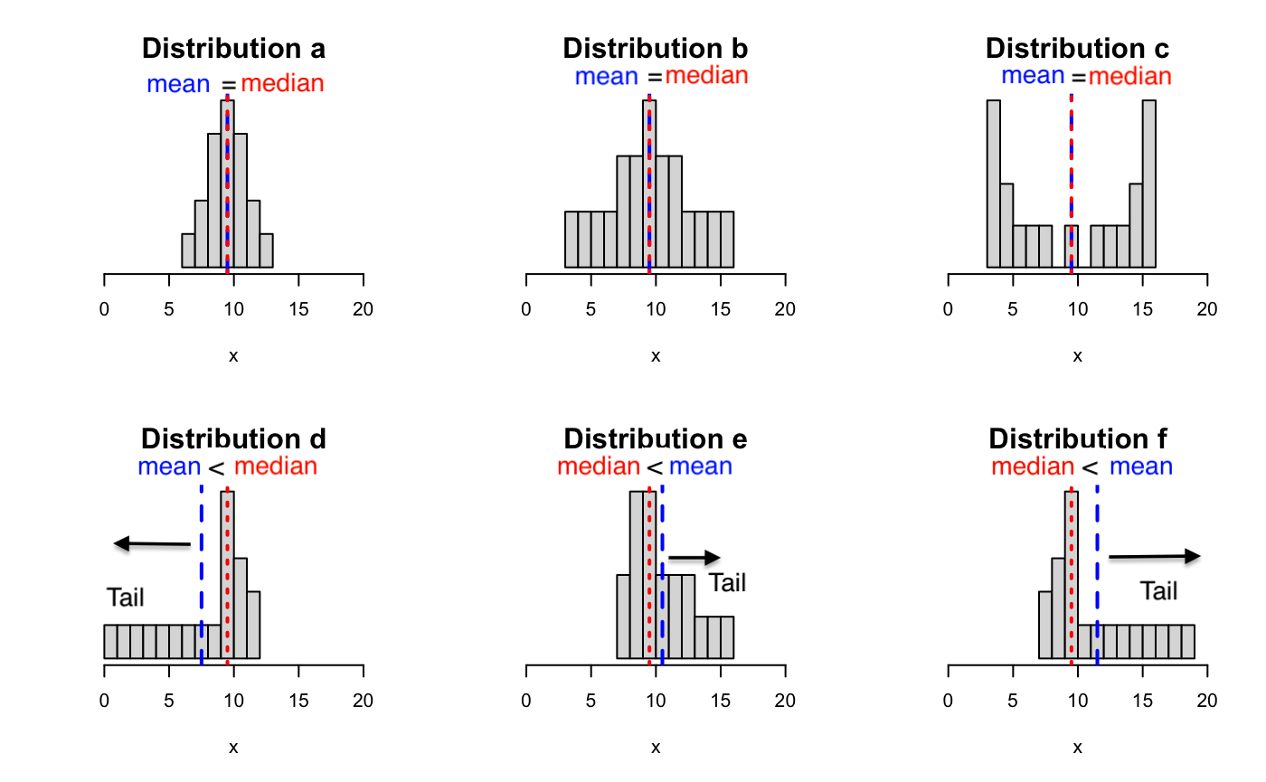
- The mean is more sensitive to outliers than the median. The mean is pulled in the direction of the tail.
- If the shape of the histogram is symmetric, then the mean is equal to the median.
- If the shape of a histogram is skewed to the left, the mean is less than the median.
- If the shape of a histogram is skewed to the right, the mean is greater than the median.
Measurements of Spread
Typical measurements of spread are:
- The range \(= \mbox{max} - \mbox{min}\).
- The advantage of the range is that it is easy to compute.
- However, the range ignores all values in the data other than the maximum and minimum values.
- The standard deviation approximately measures the average distance of all values from the mean value.
- For a sample, \(\displaystyle s = \sqrt{\dfrac{\sum_{i=1}^{n} (x_i - \bar{x})^2}{n-1}}\).
- The standard deviation takes all values into account and thus involves many calculations. We typically use technology to help!
- The command
sd(var_name)computes the sample standard deviation in R. - We use \(\color{dodgerblue}{\mathbf{s}}\) to denote a sample standard deviation.
- We use \(\color{tomato}{\mathbf{\sigma}}\) (Greek letter sigma) to denote a population standard deviation.
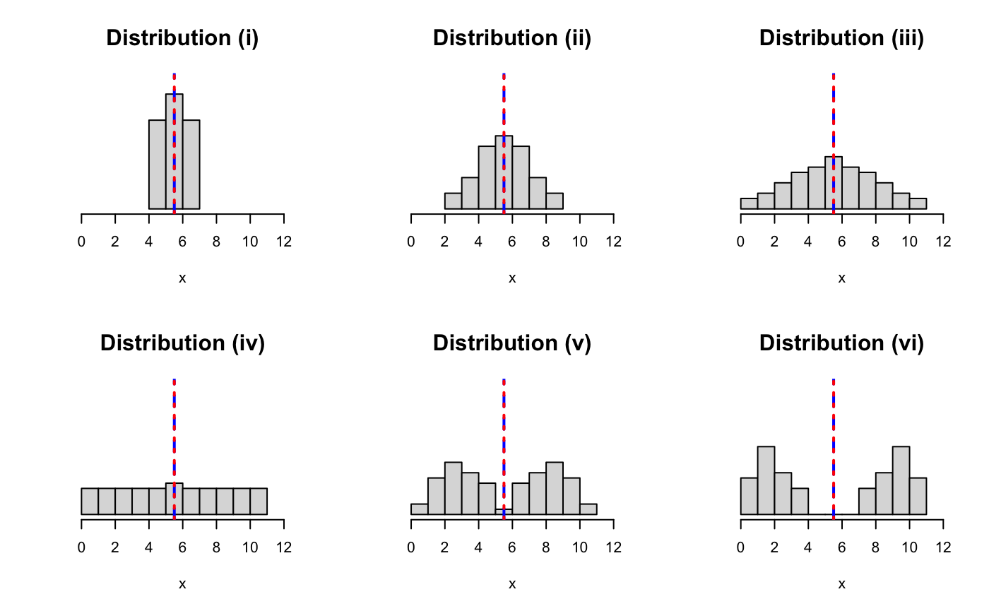
Question 12
Which of the histograms (i)-(vi) has the largest range? The smallest range?
Solution to Question 12
Question 13
Which of the histograms (i)-(vi) has the largest standard deviation? The smallest standard deviation?
Solution to Question 13
Quartiles
- The \(25^{\mbox{th}}\) percentile first quartile is denoted \(\color{dodgerblue}{\mathbf{Q_1}}\).
- In R, use the function
quantile(x, probs=0.25). - The \(75^{\mbox{th}}\) percentile third quartile is denoted \(\color{dodgerblue}{\mathbf{Q_3}}\).
- In R, use the function
quantile(x, probs = 0.75).
- In R, use the function
- The Interquartile Range (IQR)\(\color{dodgerblue}{=Q_3-Q_1}\).
- In R, use the function
IQR(x).
- In R, use the function
- The five number summary can also provide a good description of the spread of the values since we know 25% of the values fall between each consecutive pair of values. \[\color{dodgerblue}{(\mbox{min}, Q_1 , \mbox{median}, Q_3, \mbox{max} )}\]
- In R, use the function
fivenum(x)to compute the five number summary.
Question 14
Give the five number summary for the wind speed of all observations in the storms data set.
Solution to Question 14
Five Number Summaries and Boxplots
The five number summary for wind speeds is \((10, 30, 45, 65, 165)\). Below is a boxplot for this data.
- 25% of the wind speeds are between 10 and 30 knots.
- 25% of the wind speeds are between 30 and 45 knots.
- 25% of the wind speeds are between 45 and 65 knots.
- 25% of the wind speeds are between 65 and 165 knots.
boxplot(storms$wind,  # data to plot
        main = "Wind Speeds of Storms",  # main title
        xlab = "Wind Speed (in knots)",  # x-axis label
        xaxt='n',  # turn off default ticks on x-axis
        horizontal = TRUE)  # align horizontally
axis(1, at = fivenum(storms$wind))  # add tickmarks at five number summary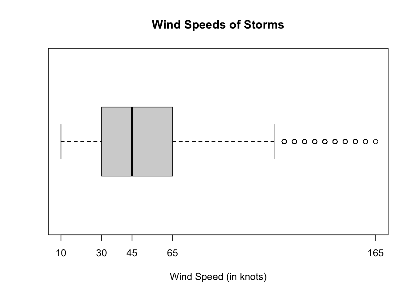
How to Read and Create Boxplots
To create a boxplot:
- Find the values of \(Q_1\), median, and \(Q_3\).
- Draw a box with edges at \(Q_1\) and \(Q_3\) and line inside the box for the median.
- Identify the upper and lower fence to classify outliers:
- Upper fence \(=Q_3 + 1.5(\mbox{IQR})\).
- Lower fence \(=Q_1 - 1.5(\mbox{IQR})\).
- Extend a line (whisker) from the lower edge of box to the smallest observation greater than the lower fence.
- Extend a line (whisker) from the upper edge of the box to the largest value that is less than the upper fence.
- The observations that are less than the lower fence or greater than the upper fence are considered outliers.
- Outlier values are marked with individual points.
Question 15
Compute the upper and lower fences for the wind speed observations in storms.
Solution to Question 15
The Empirical Cumulative Distribution Function (ecdf)
A question we often wish to explore is what proportion of values in our data are less or equal to a specified value \(x\)? To answer this question, we count the total number of observations in our data that are less than or equal to \(x\), and then divide by the total number of observations in our data.
Counting Observations with Logical Statements
To illustrate how we can count observations that satisfy a given condition, consider the a vector of 5 values: \(31\), \(33\), \(34\), \(36\), and \(38\). We store these values in the vector named test.data below. The command test.data <= 35 applies a logical test to each of the 5 values in the vector:
Is the value less than or equal to 35?
Run the code cell below and check the output to verify the test works as expected.
test.data <- c(31, 33, 34, 36, 38)  # vector of test data
test.data <= 35  # logical test
[1] TRUE TRUE TRUE FALSE FALSE- The result
TRUEis counted as 1. - The result
FALSEis counted as 0. - We can use the
sum()function to count how manyTRUEresults we have. - Running the code cell below, we verify that 3 values in
test.dataare less than or equal to 35.
sum(test.data <= 35) # sum the TRUE results[1] 3We can convert the count to a proportion by dividing by the total number of values in our data. Our vector test.data has a total of 5 observations; therefore, the proportion of values that are less than or equal to 35 is 3 out of 5 or \(0.6\). We can use the mean() to count the number of TRUE results and divide by the total number of all observations in one command to simplify the code.
mean(test.data <= 35) # total values <= 35 divided by total number of values[1] 0.6Question 16
What proportion of observations in storms$wind have a wind speed less than or equal to 50 knots?
Solution to Question 16
# what proportion of observations have wind less than or equal to 50What is the Empirical Cumulative Distribution Function?
The empirical cumulative distribution function (ecdf) is typically denoted by the notation \(\mathbf{\color{dodgerblue}{\widehat{F}(x)}}\). We read the notation \(\hat{F}\) as F hat, and we will make use of the hat notation throughout the semester.
- The input \(x\) is a value.
- The output \(\widehat{F}(x)\) of the ecdf is the proportion of values in the sample that are less than or equal to \(x\).
Recall the vector test.data contains the values \(31\), \(33\), \(34\), \(36\), and \(38\). We can express the ecdf as a piecewise function.
\[ \widehat{F}(x) = \left\{ \begin{array}{ll} 0 & x < 31 \\ 0.2 & 31 \leq x < 33 \\ 0.4 & 33 \leq x < 34 \\ 0.6 & 34 \leq x < 36 \\ 0.8 & 36 \leq x < 38 \\ 1 & x \geq 38 \end{array} \right. \]
Graphing the Empirical Cumulative Distribution Function
We can plot the ecdf using the plot.ecdf() function in R, and the resulting plot is a piecewise, step function.
plot.ecdf(test.data, col="steelblue")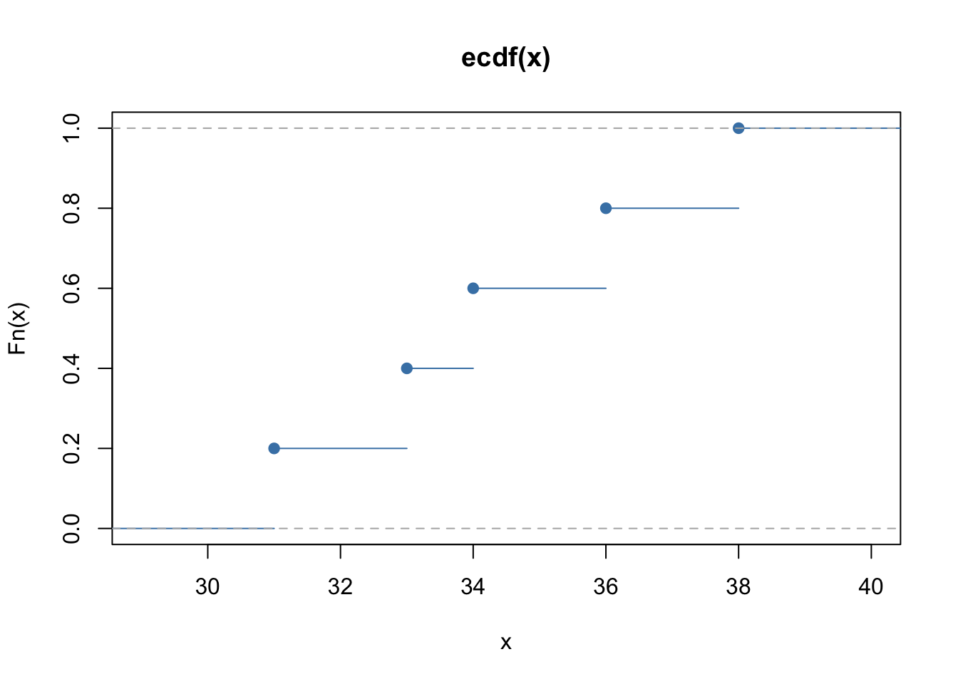
Question 17
Complete the statements below to identify some key properties of ecdf’s.
Solution to Question 17
- The minimum output value of an ecdf is ??.
- The maximum value output value of an ecdf is ??.
- The ecdf is a ?? function since as \(x\) increases, \(\widehat{F}(x)\) cannot decrease.
Question 18
Plot the empirical cumulative distribution function for the wind speeds in the storms data set and check your answer to Question 16.
Solution to Question 18
# plot the ecdf for wind speeds in stormsComparing Quantitative and Categorical Data
We have explored some of the categorical variables in the storms data set in our work with Exploring Categorical Data. We have discussed how we can summarize and plot a quantitative variable. Often in statistics we would like to compare the distribution of a quantitative variable for different classes of a categorical variable. For example, we may be interested in investigating the following:
In which month do storms have the greatest wind speed?
We first check the data type of the month variable in storms using the typeof() function.
typeof(storms$month) # check how months is stored[1] "integer"Converting a Quantitative Variable to a Categorical Variable with factor()
Months were initially stored as decimals. We converted month to an integer earlier, and we can see month is still stored as an integer. Let’s convert month to a factor so R will treat each month as a separate class.
storms$month <- factor(storms$month)  # convert month to a categorical variable
summary(storms$month)  # check summary output after converting to factor
1 4 5 6 7 8 9 10 11 12
70 66 201 779 1603 4440 7509 3077 1109 212 Side by Side Boxplots with plot()
The plot() function creates different types of plots depending on the data type and number of variables we enter.
- If
xis quantitative,plot(x)creates an index plot which is generally not too useful. - If
xis categorical,plot(x)creates a bar chart.
par(mfrow = c(1,2))  # create a 1 by 2 array of plots
plot(storms$month)  # bar chart is created for categorical data
plot(storms$wind)  # index plot is created for quantitative data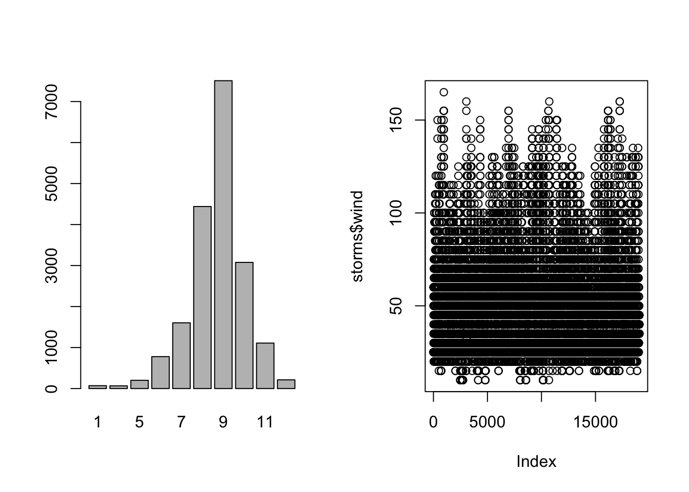
- If
xis categorical andyis quantitative,plot(y ~ x, data = [name])creates side by side boxplots, one for each class ofx. - If both
xandyare quantitative variables,plot(y ~ x, data = [name])creates a scatterplot.
par(mfrow = c(1,2))  # create a 1 by 2 array of plots
plot(wind ~ month, data = storms)  # side by side boxplots
plot(wind ~ pressure, data = storms)  # scatterplot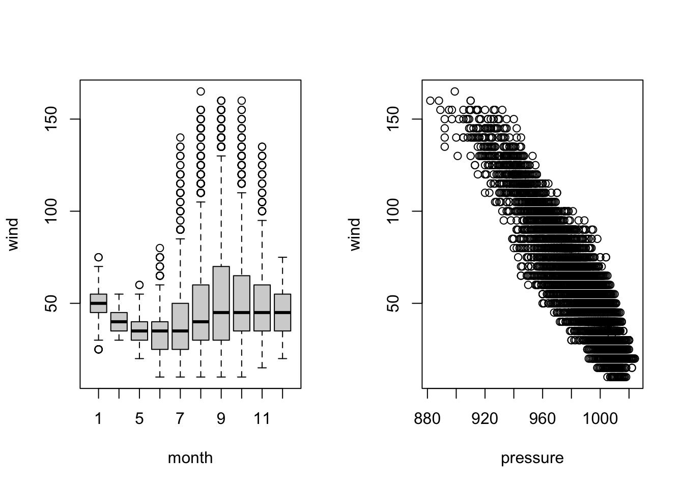
The side by side boxplots created above are hard to read since we have 12 boxplots in total. The two months with the most storms data are August and September.
How can we compare storms only in August and September?
Subsetting and Filtering Data
We can compare data for only August and September using various methods. One common method is to subset all of the data in storms into two separate data frames, one for each month. Below are three different ways we can subset data:
- Using the
subset()function in base R. - Using the
filter()function in thedplyrpackage. - Using logical statements.
Other methods exist as well.
The subset() Function in Base R
As the name implies, the subset() function in base R is a really useful function for subsetting! We can open the help documentation with ?subset to learn how to apply this function. Below are some examples of different ways we may want to subset the storms data to analyze for storms that occurred in August.
# keeps all variables for storms in August
aug <- subset(storms, month == "8")

# keeps only the wind speed variable for August storms
aug.wind <- subset(storms, select = wind, month == "8")

# drop = T drops the column name and creates a vector instead of a data frame
aug.wind.vec <- subset(storms, select = wind, month == "8", drop = T)
# we can see all variables are selected
head(aug)# A tibble: 6 × 13
name year month day hour lat long status categ…¹ wind press…² tropi…³
<chr> <int> <fct> <int> <int> <dbl> <dbl> <fct> <fct> <int> <int> <int>
1 Caro… 1975 8 24 12 22.4 -69.8 tropi… <NA> 25 1011 NA
2 Caro… 1975 8 24 18 21.9 -71.1 tropi… <NA> 25 1011 NA
3 Caro… 1975 8 25 0 21.6 -72.5 tropi… <NA> 25 1010 NA
4 Caro… 1975 8 25 6 21.2 -73.8 tropi… <NA> 25 1010 NA
5 Caro… 1975 8 25 12 20.9 -75.1 tropi… <NA> 25 1011 NA
6 Caro… 1975 8 25 18 20.6 -76.4 tropi… <NA> 25 1011 NA
# … with 1 more variable: hurricane_force_diameter <int>, and abbreviated
# variable names ¹category, ²pressure, ³tropicalstorm_force_diameter# just the wind variable is selected
head(aug.wind)# A tibble: 6 × 1
wind
<int>
1 25
2 25
3 25
4 25
5 25
6 25# wind speeds in august stored in a vector
head(aug.wind.vec)[1] 25 25 25 25 25 25Question 19
Compute the mean and median wind speed of storms in August. Compare the values of the mean and median. What does this tell us about the shape of the data?
Solution to Question 19
The filter() Function in dplyr
Using the filter function in dplyr package, we can filter out just the August observations.
- Note you need to load the
dplyrpackage with alibrary()in order to usefilter(). - We have already loaded
dplyrsince that is where thestormsdata is found. - The command below gives the same result as
subset(storms, month == "8").
aug2 <- filter(storms, month == "8")  # filter requires dplyr package
head(aug2)  # selects all variables
# A tibble: 6 × 13
name year month day hour lat long status categ…¹ wind press…² tropi…³
<chr> <int> <fct> <int> <int> <dbl> <dbl> <fct> <fct> <int> <int> <int>
1 Caro… 1975 8 24 12 22.4 -69.8 tropi… <NA> 25 1011 NA
2 Caro… 1975 8 24 18 21.9 -71.1 tropi… <NA> 25 1011 NA
3 Caro… 1975 8 25 0 21.6 -72.5 tropi… <NA> 25 1010 NA
4 Caro… 1975 8 25 6 21.2 -73.8 tropi… <NA> 25 1010 NA
5 Caro… 1975 8 25 12 20.9 -75.1 tropi… <NA> 25 1011 NA
6 Caro… 1975 8 25 18 20.6 -76.4 tropi… <NA> 25 1011 NA
# … with 1 more variable: hurricane_force_diameter <int>, and abbreviated
# variable names ¹category, ²pressure, ³tropicalstorm_force_diameterUsing Logical Statements
When writing more complex code such as for loops, it is often useful to subset data using logical statements. For example, storms[storms$month == "8", ] extracts just the rows that have a month value equal to 8.
# extract rows from storms with month equal to 8
aug.logic <- storms[storms$month == "8", ]
head(aug.logic)
# A tibble: 6 × 13
name year month day hour lat long status categ…¹ wind press…² tropi…³
<chr> <int> <fct> <int> <int> <dbl> <dbl> <fct> <fct> <int> <int> <int>
1 Caro… 1975 8 24 12 22.4 -69.8 tropi… <NA> 25 1011 NA
2 Caro… 1975 8 24 18 21.9 -71.1 tropi… <NA> 25 1011 NA
3 Caro… 1975 8 25 0 21.6 -72.5 tropi… <NA> 25 1010 NA
4 Caro… 1975 8 25 6 21.2 -73.8 tropi… <NA> 25 1010 NA
5 Caro… 1975 8 25 12 20.9 -75.1 tropi… <NA> 25 1011 NA
6 Caro… 1975 8 25 18 20.6 -76.4 tropi… <NA> 25 1011 NA
# … with 1 more variable: hurricane_force_diameter <int>, and abbreviated
# variable names ¹category, ²pressure, ³tropicalstorm_force_diameterQuestion 20
Using one of the methods above, create a data frame name sept that contains all variables for only the observations that occurred in September.
Solution to Question 20
# keeps all variables for storms in SeptemberCreating Side by Side Boxplots with boxplot
Once we have created the data frames aug and sept, we can create side by side boxplots to compare the wind speeds for storms in these two months.
# need to answer previous question first
boxplot(aug$wind, sept$wind,  # enter two vectors of data
        main = "Comparing Wind Speeds in Aug. and Sept.",   # main title
        xlab = "Wind Speed (in knots)",  # x-axis label
        horizontal = TRUE,  # align boxplots horizontally
        names = c("August", "September"),  # label each boxplot
        col = c("seagreen", "steelblue"))  # fill color for box
Question 21
In which month (August or September) are the wind speeds of storms more severe? What statistics did you use to draw your conclusion?
Solution to Question 21
Question 22
Create side by side boxplots to compare the distribution of wind speeds in July, August and September.
Solution to Question 22
Appendix: Assignment of Objects
To store a data structure in the computer’s memory we must assign it a name.
Data structures can be stored using the assignment operator <- or =.
Some comments:
- In general, both
<-and=can be used for assignment. <-and=can be used identically most of the time, but not always.- It’s safer and more conventional to use
<-for assignment. - Pressing the “Alt” and “-” keys simultaneously on a PC or Linux machine (Option and - on a Mac) will insert
<-into the R console and script files.
Why Can’t I See the Output?
In the following code, we compute the mean of a vector. Why can’t we see the result after running it?
w <- storms$wind  # wind is now stored in w
xbar.w <- mean(w)  # compute mean wind speed and assign to xbar.w
In the code cell above, the output has been stored in an object that we can refer to later.
Printing Output to Screen
Once an object has been assigned a name, it can be printed by executing the name of the object or using the print function or just entering the object name.
xbar.w  # print the mean wind speed to screen
print(xbar.w)  # print a different way
Assigning and Printing An Object At Once
Another nice way to both execute, store, and print the output of a command is the parentheses ( ) method.
(sd.w <- sd(w)) # using ( ) around a command will execute, store and print outputSometimes you want to see the result of a code cell, and sometimes you will not.

Statistical Methods: Exploring the Uncertain by Adam Spiegler is licensed under a Creative Commons Attribution-NonCommercial-ShareAlike 4.0 International License.