# use code to help with the calculations5.5: Parametric Confidence Intervals for Proportions
![]()
Public Opinion Polls
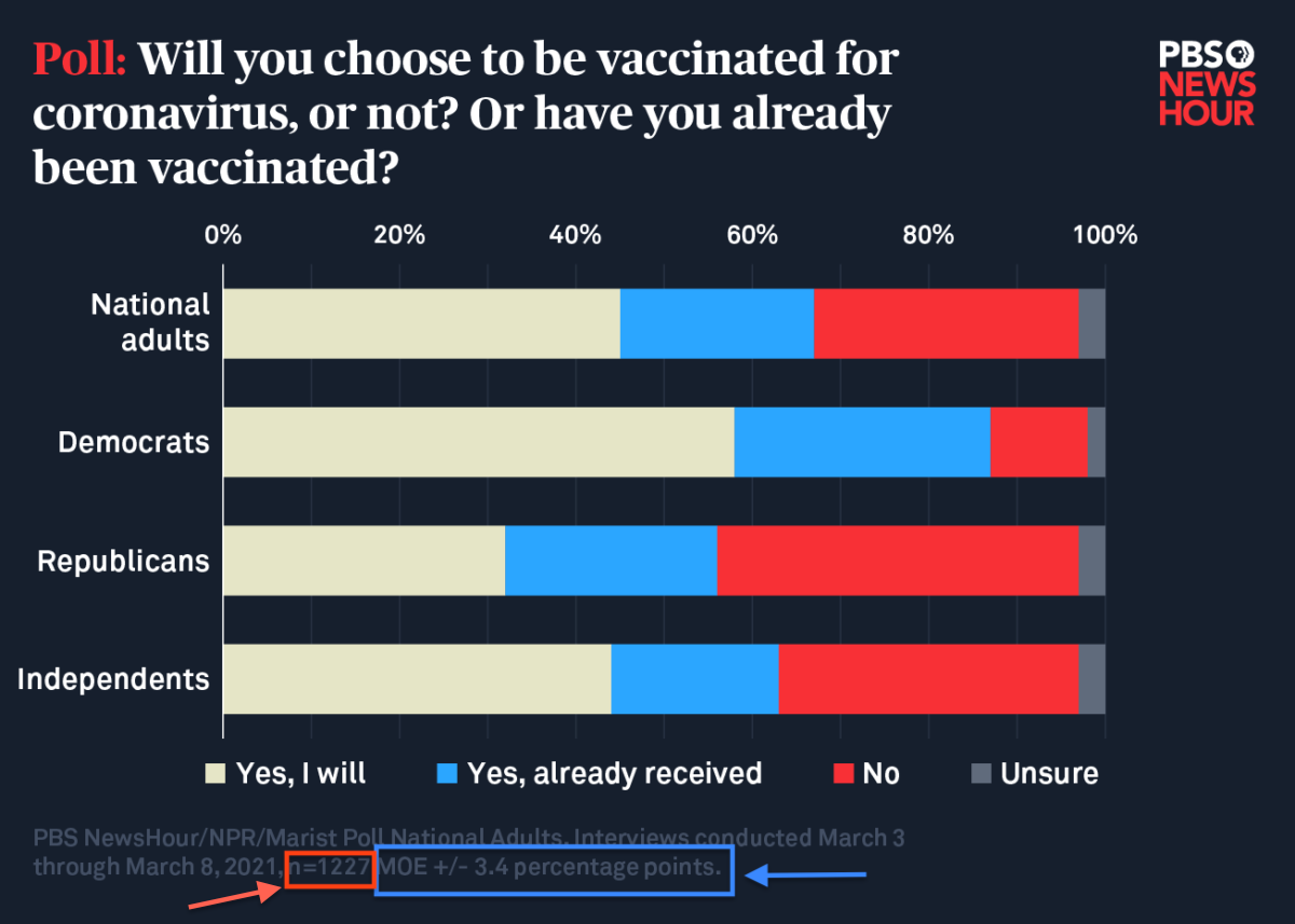
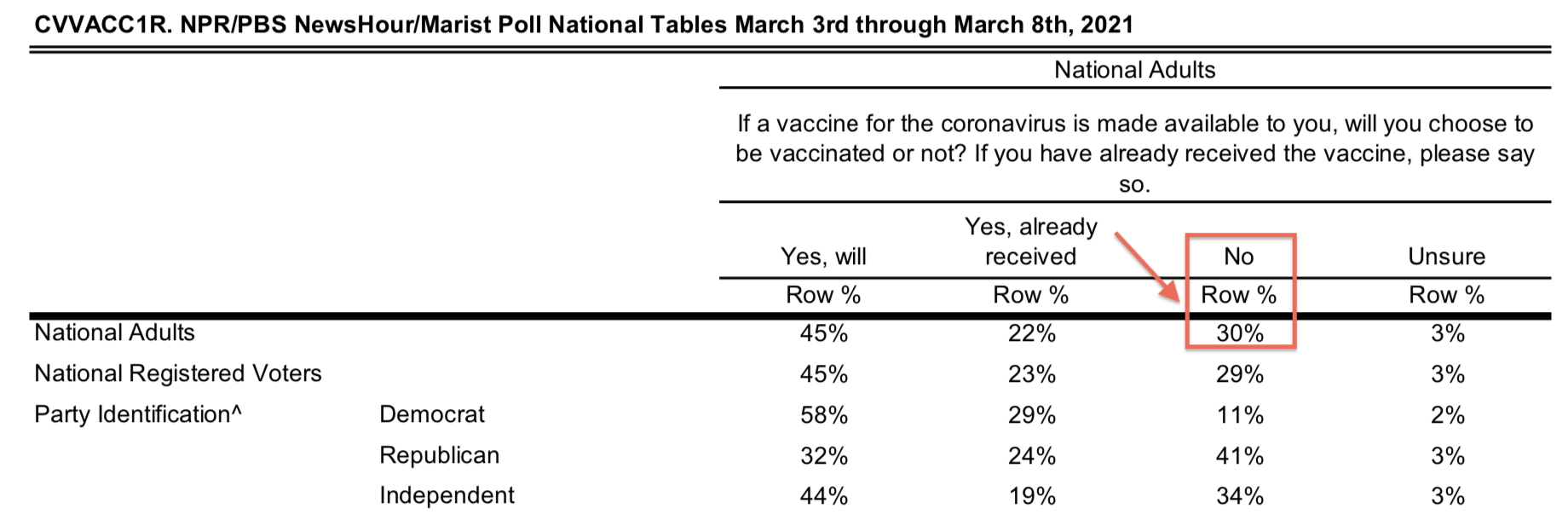
Confidence intervals are frequently used when polling public opinion. Rather than give a point estimate alone, poll results are typically given along with a margin of error corresponding to a specified confidence level, which is typically 95%. For example, summarized in the bar plot and table below are the results of a PBS NewsHour/NPR/Marist poll1 that surveyed \({\color{tomato}{n=1,\!227}}\) randomly selected adults in the US and gauged their opinions on how the US is handling the COVID pandemic approximately one year after the initial outbreak in the United States.
Question 1
Based on the poll summaries above, approximately what proportion of ALL adults in the US do NOT plan to get vaccinated?
Solution to Question 1
A General Summary of Confidence Intervals
A confidence interval is an interval estimate for a population parameter with a rate of success given by the confidence level of the interval. We can construct confidence intervals for all sorts of statistics, and we can use confidence intervals as a tool for analyzing possible associations between two different variables. In general, a confidence interval has three components:
- A point estimate is calculated from a sample.
- A confidence level is chosen.
- A margin of error (MoE) to account for the uncertainty due to sampling.
- The MoE depends on the confidence level that is chosen.
- Careful, the MoE is different from the standard error, but they are related!
- The MoE is a multiple of the standard error, SE.
If we want to construct a confidence interval estimate for parameter \(\theta\), then we have
\[({\color{dodgerblue}{\mbox{point estimate}}}) - {\color{tomato}{\mbox{MoE}}} < \theta < ({\color{dodgerblue}{\mbox{point estimate}}}) + {\color{tomato}{\mbox{MoE}}}.\]
All confidence intervals have this same general structure that we can construct using similar steps:
- Choose a point estimate.
- Using the CLT, estimate the standard error.
- Based on the confidence level, find the appropriate multiple (\(z_{\alpha/2}\) or \(t_{\alpha/2}\)).
- The margin of error (MoE) is the of product the SE and either \(z_{\alpha/2}\) or \(t_{\alpha/2}\).
Confidence Intervals for a Single Mean with Known \(\sigma^2\)
If we would like to estimate a population mean \(\mu\) of a population that has known variance \(\sigma^2\), we can pick a random sample of \(n\) values from the population. As long as the sample is large enough or symmetric, we have:
- A reasonable point estimate is the corresponding sample mean, \(\bar{x}\).
- From CLT, the standard error is \(\mbox{SE} = \frac{\sigma}{\sqrt{n}}\).
- Using the standard normal distribution, find the value of \(z_{\alpha/2}\).
- The MoE \(= z_{\alpha/2} \cdot \frac{\sigma}{\sqrt{n}}\).
\[ {\color{dodgerblue}{\overline{X}}} - {\color{tomato}{z_{\alpha/2} \cdot \frac{\sigma}{\sqrt{n}}}} < \mu < {\color{dodgerblue}{\overline{X}}} + {\color{tomato}{z_{\alpha/2} \cdot \frac{\sigma}{\sqrt{n}}}} .\]
Confidence Intervals for a Single Mean with Unknown \(\sigma^2\)
If we would like to estimate a population mean \(\mu\) of a population that has unknown variance \(\sigma^2\), we can pick a random sample of \(n\) values from the population. As long as the sample is large enough or symmetric, we have:
- A reasonable point estimate is the corresponding sample mean, \(\bar{x}\).
- We use CLT, plugging \(s\) in place of \(\sigma\), to get \(\mbox{SE} = \frac{{\color{mediumseagreen}{s}}}{\sqrt{n}}\).
- Using a \(t\)-distribution, find the value of \({\color{mediumseagreen}{t_{\alpha/2}}}\).
- The MoE \(= {\color{mediumseagreen}{t_{\alpha/2}}} \cdot \frac{{\color{mediumseagreen}{s}}}{\sqrt{n}}\).
\[{\color{dodgerblue}{\overline{X}}} - {\color{tomato}{t_{\alpha/2} \cdot \frac{s}{\sqrt{n}}}} < \mu < {\color{dodgerblue}{\overline{X}}} + {\color{tomato}{t_{\alpha/2} \cdot \frac{s}{\sqrt{n}}}} .\]
Confidence Interval for a Difference in Two Means
If we would like to estimate the difference in means from two independent populations that have unknown variances, we can pick random samples of sizes \(n_1\) and \(n_2\) from each respective population. As long as the samples are large enough or symmetric, we have:
- A reasonable point estimate is the corresponding difference in sample means, \(\bar{x}_1 - \bar{x}_2\).
- We use CLT, plugging \(s_1\) and \(s_2\) in place of \(\sigma_1\) and \(\sigma_2\), to get
\[{\color{mediumseagreen}{\mbox{SE} = \sqrt{ \frac{s_1^2}{n_1} + \frac{s_2^2}{n_2}}}}.\]
- Using a \(t\)-distribution, find the value of \({\color{mediumseagreen}{t_{\alpha/2}}}\).
- The MoE \(= {\color{mediumseagreen}{t_{\alpha/2}}} \cdot \sqrt{ \frac{{\color{mediumseagreen}{s_1}}^2}{n_1} + \frac{{\color{mediumseagreen}{s_2}}^2}{n_2}}\).
\[\left( {\color{dodgerblue}{\overline{X}-\overline{Y}}} \right) - {\color{tomato}{t_{\alpha/2} \cdot \sqrt{ \frac{s_1^2}{n_1} + \frac{s_2^2}{n_2}}}} < \mu_1 - \mu_2 < \left( {\color{dodgerblue}{\overline{X}-\overline{Y}}} \right) + {\color{tomato}{t_{\alpha/2} \cdot \sqrt{ \frac{s_1^2}{n_1} + \frac{s_2^2}{n_2}}}} .\]
Question 2
We would like to estimate the parameter \(p\), the proportion of all adults in the US that do not plan on getting vaccinated. From the vaccination poll in Question 1, we have one random sample of 1,227 adults. From our sample, we observe that 30% said they do not intend to get vaccinated. Let’s apply the same general process summarized above to construct a 95% confidence interval to estimate the proportion of all adults in the US that do not plan on getting vaccinated.
Question 2a
Based on the sample of polled adults, what is a reasonable point estimate for \(p\), the proportion of all adults in the US that do not plan on getting vaccinated?
Solution to Question 2a
Question 2b
Using the Central Limit Theorem for proportions, estimate the standard error for the sampling distribution of sample proportions.
Tip
To calculate the standard error, we need to know the population proportion \(p\). Plug an appropriate sample statistic in place of \(p\) to estimate the standard error.
Solution to Question 2b
Question 2c
Next, we identify the value (\(z_{\alpha/2}\) or \(t_{\alpha/2}\)) we multiply the standard error by to get the margin of error. For proportions, as long as the the sample is large enough, a normal distribution is an accurate model for the underlying sampling distribution.
From the poll in Question 1, we have \(n=1227\). Since we do not know \(p\), we substitute \(\hat{p} = 0.3\) instead. Since both \(n\hat{p} \geq 10\) and \(n(1-\hat{p}) \geq 10\), we can use a normal distribution to calculate the margin of error for the confidence interval.
What is the value of \(z_{\alpha/2}\) for a 95% confidence interval for a proportion?
Solution to Question 2c
Question 2d
Based on your previous answers in Question 2, give a 95% confidence interval to estimate \(p\), the proportion of all adults in the US that do not plan on getting vaccinated.
Solution to Question 2d
Question 2e
Interpret the practical meaning of your confidence interval in Question 2d in the context of COVID vaccinations in the US.
Solution to Question 2e
Wald Confidence Interval for a Proportion
The Wald confidence interval for a proportion is given by
\[{\large \boxed{ \mbox{Wald:} \qquad {\color{tomato}{\hat{p}}} - z_{\alpha/2} \cdot \sqrt{ \frac{{\color{tomato}{\hat{p}}}(1-{\color{tomato}{\hat{p}}})}{n}} < p < {\color{tomato}{\hat{p}}} + z_{\alpha/2} \cdot \sqrt{ \frac{{\color{tomato}{\hat{p}}}(1-{\color{tomato}{\hat{p}}})}{n}}}}\]
We use the plug-in principle and use \(\hat{p}\) for the unknown value of \(p\) when calculating the standard error.
- The advantage of this estimate is we can do it by hand.
- The downside is we have introduced additional uncertainty using \(\hat{p}\) in place of \(p\) when estimating the standard error.
We use the standard normal distribution to identify \({\color{mediumseagreen}{z_{\alpha/2}}}\) when finding the margin of error since we are using a continuous distribution (proportions) to approximate a binomial distribution (counts).
Agresti-Coull Confidence Interval for a Proportion
When constructing a Wald confidence interval for a proportion, we use the sample proportion \(\hat{p}\) as an estimator for \(p\). The sample proportion is a very reasonable and intuitive point estimate. In addition, \(\hat{p}\) is an unbiased estimator for \(p\). However, there are many other estimators that could make sense to use in place of the parameter \(p\), and there are other properties of estimators we should take into account. In particular, using a less precise estimator such as \(\hat{p}\) results in a larger margin of error in the confidence interval compared to some other estimators.
When studying properties of estimators, we considered another estimator for the parameter \(p\), namely \({\color{tomato}{\tilde{p} = \frac{X+2}{n+4}}}\), where \(X\) denotes the number of “successes”. Comparing estimators \(\hat{p}\) and \(\tilde{p}\), we discovered that:
- The modified sample proportion \({\color{tomato}{\tilde{p}}}\) is slightly biased but more precise than \(\hat{p}\) as long as \(p\) is not close to either \(0\) or \(1\).
- Thus, the confidence interval using \({\color{tomato}{\tilde{p}}}\) will have a smaller margin of error than using \(\hat{p}\) when \(p\) is not close to either \(0\) or \(1\).
The Agresti-Coull confidence interval for a proportion is
\[{\large \boxed{ \mbox{Agresti-Coull:} \qquad {\color{tomato}{\tilde{p}}} - z_{\alpha/2} \left( \sqrt{ \frac{{\color{tomato}{\tilde{p}}}(1-{\color{tomato}{\tilde{p}}})}{{\color{dodgerblue}{n+4}}}} \right) < p < {\color{tomato}{\tilde{p}}} + z_{\alpha/2} \left( \sqrt{ \frac{{\color{tomato}{\tilde{p}}}(1-{\color{tomato}{\tilde{p}}})}{{\color{dodgerblue}{n+4}}}} \right)}}.\]
Question 3
Using the same poll from Question 1, find a 95% confidence interval for the proportion of all adults in the US that do not plan to get vaccinated using the Agresti-Coull confidence interval for a proportion.
Solution to Question 3
Score Confidence Interval For a Proportion
From the CLT for proportions, we have \(\widehat{P} \sim N \left( \mu_{\widehat{P}} , \sigma_{\widehat{P}} \right) = N\left( p, \sqrt{\frac{ p (1-p)}{n}} \right)\). A standardized sample proportion has \(z\)-score \(z = \frac{\hat{p} - p}{\sqrt{\frac{ p (1-p)}{n}}}\). Thus, for confidence level \(CL\), we have
\[P \left( -z_{\alpha/2} < \frac{\hat{p} -\color{tomato}{p}}{\sqrt{\frac{\color{tomato}{p}(1-\color{tomato}{p})}{n}}} < z_{\alpha/2} \right) =CL.\]
In the equation above, the unknown population parameter \(p\) is in red. All the other values (\(\hat{p}\), \(n\), and \(z_{\alpha/2}\)) in the formula are known values. Given a confidence level, we can algebraically solve for the cutoff values for \({\color{tomato}{p}}\) by solving the equations:
\[\dfrac{\hat{p} -{\color{tomato}{p}}}{\sqrt{\dfrac{{\color{tomato}{p}}(1-{\color{tomato}{p}})}{n}}} = z_{\alpha/2} \qquad \mbox{and} \qquad \dfrac{\hat{p} - {\color{tomato}{p}}}{\sqrt{\dfrac{{\color{tomato}{p}}(1-{\color{tomato}{p})}}{n}}} = -z_{\alpha/2}\]
Score Confidence Interval Formulas
The confidence interval estimate resulting from the algebraic solution is called the score confidence interval for a proportion. The algebraic work involved in solving the equations above is provided in the Appendix. The corresponding lower (\(L\)) and upper (\(U\)) cutoffs are:
\[\begin{aligned} &L= \dfrac{\hat{p} + \dfrac{z_{\alpha/2}^2}{2n} - z_{\alpha/2} \cdot \sqrt{ \dfrac{\hat{p}(1-\hat{p})}{n} + \dfrac{z_{\alpha/2}^2}{4n^2}}}{1+ \dfrac{z_{\alpha/2}^2}{n}} \\ \\ &U= \dfrac{\hat{p} + \dfrac{z_{\alpha/2}^2}{2n} + z_{\alpha/2} \cdot \sqrt{ \dfrac{\hat{p}(1-\hat{p})}{n} + \dfrac{z_{\alpha/2}^2}{4n^2}}}{1+ \dfrac{z_{\alpha/2}^2}{n}} \end{aligned}\]
- Pro: There is no additional uncertainty beyond the initial variability in sampling.
- Con: The formulas are quite complicated. Calculating by hand is not really practical.
- Typically we use technology to calculate score confidence intervals.
Score Confidence Intervals in R
R has a built in function prop.test()$conf.int that calculates a score confidence interval for a proportion.
- In R, use the command
prop.test(X, n, conf.level = CL, correct = FALSE)$conf.int- \(X\) denotes the number of “successes” observed in the sample.
- \(n\) denotes the total number of observations in the sample.
CLis a chosen confidence level (as a proportion).- The option
correct = FALSEmeans no continuity correction is applied.
Question 4
Using the poll data in Question 1, find a 95% score confidence interval for the proportion of all adults in the US that do not plan to get vaccinated by completing the prop.test() command in the code cell below.
Solution to Question 4
prop.test(??, ??, conf.level = ??, correct = FALSE)$conf.int
Checking Your Solution to Question 4
Based on the polling sample data, enter the values for X, n, and z.star in the first code cell below. Then run the code cell.
##################################################
# Replace the ?? in the three lines of code below
# with appropriate values or commands
##################################################
X <- ??  # number of successes in sample (do not plan to get vax)
n <- ??  # sample size
z.star <- ??  # find z_alpha/2 for 95% confidence level
Next, run the code cell below to calculate the upper and lower cutoffs for a 95% score confidence interval for a proportion.
#########################################
# first run the code cell above
# nothing to edit in this code cell
# run as is
#########################################
phat <- X/n  # Compute sample proportion

# Computes Cutoffs for Score Confidence Interval
lower.score95 <- (phat+z.star^2/(2*n) -
                z.star*sqrt( (phat*(1-phat))/n + z.star^2/(4*n^2) ) )/(1+z.star^2/n)
upper.score95 <- (phat+z.star^2/(2*n) +
                z.star*sqrt( (phat*(1-phat))/n + z.star^2/(4*n^2) ) )/(1+z.star^2/n)

# Print cutoffs to screen
lower.score95
upper.score95
Applying the Continuity Correction
In our construction of a score confidence interval, we have used a normal distribution to estimate a discrete (binomial) distribution. Recall when using a continuous, normal distribution to approximate a discrete, binomial distribution (as with the Central Limit Theorem for proportions), we miss some area under the curve resulting in an underestimate. We can improve estimates resulting from using a normal distribution instead of a binomial distribution by applying a continuity correction.
Similarly, we can obtain more a more accurate score confidence interval for a proportion by applying a continuity correction. The Appendix explains how the continuity correction is applied and provides the corresponding formulas. In practice, we can simply change the correct = FALSE option in prop.test()$conf.int to correct = TRUE.
prop.test(X, n, conf.level = CL, correct = TRUE)$conf.int- The default for
prop.testif nocorrectoption is specified iscorrect = TRUE. - Applying the continuity correction results in a more precise confidence interval.
Applying the Continuity Correction in Code
Below we perform the direct calculations using the continuity correction formulas derived in the Appendix.
##############################################
# Be sure you have run previous code cells
# And have already defined X, n, and z.star
# Run this code cell without any edits needed
##############################################

# Continuity corrections applied to sample proportion
cc.phat.L <- (X - 0.5)/n
cc.phat.U <- (X + 0.5)/n

# Plugged into formulas for Score Conf Interval
cc.lower <- (cc.phat.L + z.star^2/(2*n) -
            z.star*sqrt( (cc.phat.L*(1-cc.phat.L))/n + z.star^2/(4*n^2) ) )/(1+z.star^2/n)
cc.upper <- (cc.phat.U + z.star^2/(2*n) +
            z.star*sqrt( (cc.phat.U*(1-cc.phat.U))/n + z.star^2/(4*n^2) ) )/(1+z.star^2/n)

# Print results to screen to check
cc.lower
cc.upper
In the code cell below, we apply the continuity correction using the correct = TRUE option in prop.test() to compare with the previous result.
prop.test(368, 1227, conf.level = 0.95, correct = TRUE)$conf.int
A Difference in Two Proportions
Central Limit Theorem for \(\widehat{P}_1 - \widehat{P}_2\)
For a difference in two proportions, we can derive a Central Limit Theorem to model the sampling distribution for the difference in two sample proportions, \(\widehat{P}_1 - \widehat{P}_2\). See the Appendix for a proof of the CLT for a difference in two proportions which is stated below:
\[\widehat{P}_1 - \widehat{P}_2 \sim N \left( \mu_{\widehat{P}_1 - \widehat{P}_2} , \mbox{SE}(\widehat{P}_1 - \widehat{P}_2) \right) = N \left( p_1 - p_2 , \sqrt{\frac{p_1(1-p_1)}{n_1} + \frac{p_2(1-p_2)}{n_2}} \right).\]
Confidence Interval for \(\widehat{P}_1 - \widehat{P}_2\)
We can modify the Wald confidence interval to give an approximation for a confidence interval for a difference in two proportions
- The point estimate is the difference in the two sample proportions, \(\color{dodgerblue}{\hat{p}_1 - \hat{p}_2}\).
- The standard error we estimate by plugging \(\hat{p}_1\) and \(\hat{p}_2\) in place of \(p_1\) and \(p_2\) in the formula for the standard error from the Central Limit Theorem:
\[\mbox{SE} \left( \widehat{P}_1 - \widehat{P}_2 \right) = \sqrt{ \frac{p_1(1-p_1)}{n_1} + \frac{p_2(1-p_2)}{n_2}} \approx \sqrt{ \frac{{\color{mediumseagreen}{\hat{p}_1}}(1-{\color{mediumseagreen}{\hat{p}_1}})}{n_1} + \frac{{\color{mediumseagreen}{\hat{p}_2}}(1-{\color{mediumseagreen}{\hat{p}_2}})}{n_2}}\]
- Since we are using a continuous distribution (proportions) to approximate a binomial distribution (counts), we use the standard normal distribution to identify \(z_{\alpha/2}\) to find the margin of error.
- Note: A normal distribution is an accurate model assuming all four of the conditions are true: \(n_1 p_1 \geq 10\), \(n_1(1-p_1) \geq 10\), \(n_2 p_2 \geq 10\), and \(n_2(1-p_2) \geq 10\).
- Thus, we have a Wald confidence interval for a difference in proportions.
\[({\color{dodgerblue}{\hat{p}_1 - \hat{p}_2}}) - {\color{tomato}{z_{\alpha/2} \cdot \sqrt{ \dfrac{\hat{p}_1(1-\hat{p}_1)}{n_1} + \dfrac{\hat{p}_2 (1-\hat{p}_2) }{n_2}}}} < p_1-p_2 < ({\color{dodgerblue}{\hat{p}_1 - \hat{p}_2}}) + {\color{tomato}{z_{\alpha/2} \cdot \sqrt{ \dfrac{\hat{p}_1(1-\hat{p}_1)}{n_1} + \dfrac{\hat{p}_2 (1-\hat{p}_2) }{n_2}}}}\]
A Wald Confidence Interval for \(p_1 - p_2\) Using prop.test()
The formulas above give a Wald confidence intervals for a difference in two proportions. Be aware there are other variations of confidence intervals for a difference in two proportions similar to the Agresti-Coull and score confidence intervals.
In R, the command
prop.test(c(x1, x2), c(n1, n2), conf.level = CL, correct = FALSE)$conf.int
computes a Wald confidence interval for a difference in two proportions without a continuity correction applied. If we want to apply a continuity correction2, we use the option correct = TRUE.
Note
In R, the prop.test() function uses different methods depending on whether the confidence interval is for a single proportion or a difference in two proportions.
- For a single proportion,
prop.test()gives a score confidence interval. - For a difference in two proportions,
prop.test()gives a Wald confidence interval.
Question 5
Using the data below collected from the poll in Question 1, construct a 90% Wald confidence interval for the difference in the proportion of all Democrats and the proportion of all Republicans that do not plan to be vaccinated.
| Party | Yes, will | Yes, already | No | Unsure | Total |
|---|---|---|---|---|---|
| Democrat | 213 | 108 | 40 | 7 | 368 |
| Republican | 93 | 70 | 120 | 9 | 292 |
| Total | 306 | 178 | 160 | 16 | 660 |
Solution to Question 5
# use code cell to help
Summarizing Results of Confidence Intervals
| Parameter(s) of Interest | Point Estimate | Distribution | Margin of Error |
|---|---|---|---|
| A single mean (\(\sigma^2\) known) |
\(\bar{x}\) | \(N(0,1)\) | \(z_{\alpha/2} \cdot \dfrac{\sigma}{\sqrt{n}}\) |
| A single mean (\(\sigma^2\) unknown) |
\(\bar{x}\) | \(t\)-dist | \({\color{mediumseagreen}{t_{\alpha/2}}} \cdot \dfrac{{\color{tomato}{s}}}{\sqrt{n}}\) |
| A difference in two means (with unknown variances) |
\(\bar{x}_1 - \bar{x}_2\) | \(t\)-dist | \({\color{mediumseagreen}{t_{\alpha/2}}} \cdot \sqrt{ \dfrac{{\color{tomato}{s_1}}^2}{n_1} + \dfrac{{\color{tomato}{s_2}}^2}{n_2}}\) |
| Wald for single proportion | \(\hat{p}=\dfrac{X}{n}\) | \(N(0,1)\) | \(z_{\alpha/2} \cdot \sqrt{ \dfrac{{\color{tomato}{\widehat{p}}}(1-{\color{tomato}{\widehat{p}}})}{n}}\) |
| Agresti-Coull for single proportion | \(\tilde{p}=\dfrac{X+2}{n+4}\) | \(N(0,1)\) | \(z_{\alpha/2} \cdot \sqrt{ \dfrac{{\color{tomato}{\tilde{p}}}(1-{\color{tomato}{\tilde{p}}})}{{\color{dodgerblue}{n+4}}}}\) |
| Wald for a difference in two proportions |
\(\hat{p}_1 - \hat{p}_2\) | \(N(0,1)\) | \(z_{\alpha/2} \cdot \sqrt{ \dfrac{{\color{tomato}{\hat{p}_1}}(1-{\color{tomato}{\hat{p}_1}})}{n_1} + \dfrac{{\color{tomato}{\hat{p}_2}}(1-{\color{tomato}{\hat{p}_2}})}{n_2}}\) |
A Note About Sample Sizes
For a single mean, we can use the CTL to construct a parametric confidence interval as long as:
- Either the population is symmetric or \(n \geq 30\).
- If the sample is symmetric, we can assume the population is symmetric.
For a difference in two means , we can use the CTL to construct a parametric confidence interval as long as:
- Population 1 is either symmetric or \(n_1 \geq 30\), and
- Population 2 is either symmetric or \(n_2 \geq 30\).
For a single proportion, we can use the CTL to construct a parametric confidence interval as long as:
- Both \(n\hat{p} \geq 10\) and \(n(1-\hat{p}) \geq 10\).
For a difference in two proportions, we can use the CTL to construct a parametric confidence interval as long as:
- All of \(n_1\hat{p}_1 \geq 10\), \(n_1(1-\hat{p}_1) \geq 10\), \(n_2\hat{p}_2 \geq 10\), and \(n_2(1-\hat{p}_2) \geq 10\) are satisfied.
Useful R Functions
In R, we have the functions:
t.test()$conf.intconstructs a \(t\)-confidence interval for a single or difference in two means.prop.test()$conf.intconstructs a score confidence interval for a single proportion.prop.test()$conf.intconstructs a Wald confidence interval for a difference in two proportions.
Appendix
Deriving the Score Confidence Interval Formulas
Let \(X \sim \mbox{Binom}(n,p)\) and consider the distribution of sample proportions, \(\widehat{P} = \frac{X}{n}\). From the CLT for proportions we know \(\widehat{P} \sim N \left( p, \sqrt{\frac{p(1-p)}{n}} \right)\). Thus, for confidence level CL, we have
\[P(-z_{\alpha/2}< Z < z_{\alpha/2}) = P \left( -z_{\alpha/2} < \frac{\hat{p} -{\color{tomato}{p}}}{\sqrt{\frac{{\color{tomato}{p}}(1-{\color{tomato}{p}})}{n}}} < z_{\alpha/2} \right) =CL.\]
The upper cutoff, \(U\) is a value for \({\color{tomato}{p}}\) such that
\[\dfrac{\hat{p} -{\color{tomato}{p}}}{\sqrt{\dfrac{{\color{tomato}{p}}(1-{\color{tomato}{p}})}{n}}} = z_{\alpha/2}.\]
To solve for \({\color{tomato}{p}}\), we multiply both sides of the equation above by \(\sqrt{\dfrac{{\color{tomato}{p}}(1-{\color{tomato}{p}})}{n}}\) and then square both sides giving
\[\big( \hat{p} - {\color{tomato}{p}} \big)^2 = (z_{\alpha/2})^2 \left( \frac{{\color{tomato}{p}}(1-{\color{tomato}{p}})}{n} \right).\]
Next we distribute terms on both sides of the equation and have
\[\hat{p}^2 - 2 {\color{tomato}{p}}\hat{p} + {\color{tomato}{p}}^2 = {\color{tomato}{p}} \left( \frac{z_{\alpha/2}^2}{n} \right) - {\color{tomato}{p}}^2 \left( \frac{z_{\alpha/2}^2}{n} \right).\]
We have a quadratic equation for the unknown \({\color{tomato}{p}}\). We group all like terms together on one side of the equation,
\[{\color{dodgerblue}{\left( 1+ \frac{z_{\alpha/2}^2}{n} \right)}} p^2 + {\color{tomato}{\left(-2\hat{p}-\frac{z_{\alpha/2}^2}{n} \right)}} p + {\color{mediumseagreen}{\hat{p}^2}} = {\color{dodgerblue}{a}}p^2 + {\color{tomato}{b}} p + {\color{mediumseagreen}{c}} = 0.\] We use the quadratic formula to solve for \(p\). The quadratic equation has two real solutions, the larger of the two solution is the upper limit for a 95% score confidence interval
\[{\large \boxed{ U = \frac{ \hat{p} + \dfrac{z_{\alpha/2}^2}{2n} + z_{\alpha/2} \cdot \sqrt{ \dfrac{\hat{p}(1-\hat{p})}{n} + \dfrac{z_{\alpha/2}^2}{4n^2}}}{1+\dfrac{z_{\alpha/2}^2}{n}}}}\]
The smaller of the two solutions is the lower cutoff, \(L\)
\[{\large \boxed{ L = \frac{ \hat{p} + \dfrac{z_{\alpha/2}^2}{2n} - z_{\alpha/2} \cdot \sqrt{ \dfrac{\hat{p}(1-\hat{p})}{n} + \dfrac{z_{\alpha/2}^2}{4n^2}}}{1+\dfrac{z_{\alpha/2}^2}{n}}}}\]
We also consider the equation
\[\dfrac{\hat{p} -{\color{tomato}{p}}}{\sqrt{\dfrac{{\color{tomato}{p}}(1-{\color{tomato}{p}})}{n}}} = -z_{\alpha/2}.\]
If we multiply both sides of the equation above by \(\sqrt{\dfrac{{\color{tomato}{p}}(1-{\color{tomato}{p}})}{n}}\) and then square both sides, we get
\[\big( \hat{p} - {\color{tomato}{p}} \big)^2 = (-z_{\alpha/2})^2 \left( \frac{{\color{tomato}{p}}(1-{\color{tomato}{p}})}{n} \right).\]
The resulting equation is the same as with the first case we solved. Thus, solving the equation above gives the same expressions for \(U\) and \(L\).
Applying a Continuity Correction to a Score Confidence Interval
Recall, when using a normal distribution to approximate a discrete, binomial distribution \(X \sim \mbox{Binom}(n,p)\), we can improve the estimate by using a continuity correction.
In the case of a score confidence interval for a proportion, the continuity correction is applied as follows:
- In the formula for the corrected lower cutoff \(L^*\), we use the corrected sample proportion \({\color{dodgerblue}{\hat{p}_L^*= \dfrac{X-0.5}{n}}}\).
- In the formula for the corrected upper cutoff \(U^*\), we use the corrected sample proportion \({\color{tomato}{\hat{p}_U^* = \dfrac{X+0.5}{n}}}\).
\[\begin{aligned} &L^* = \dfrac{{\color{dodgerblue}{\hat{p}_L^*}} + \dfrac{z_{\alpha/2}^2}{2n} - z_{\alpha/2} \cdot \sqrt{ \dfrac{{\color{dodgerblue}{\hat{p}_L^*}}(1-{\color{dodgerblue}{\hat{p}_L^*}})}{n} + \dfrac{z_{\alpha/2}^2}{4n^2}}}{1+ \dfrac{z_{\alpha/2}^2}{n}} \\ \\ &U^* = \dfrac{{\color{tomato}{\hat{p}_U^*}} + \dfrac{z_{\alpha/2}^2}{2n} + z_{\alpha/2} \cdot \sqrt{ \dfrac{{\color{tomato}{\hat{p}_U^*}}(1-{\color{tomato}{\hat{p}_U^*}})}{n} + \dfrac{z_{\alpha/2}^2}{4n^2}}}{1+ \dfrac{z_{\alpha/2}^2}{n}} \end{aligned}\]
CLT: Difference in Two Proportions
Let \(X_1 \sim \mbox{Binom}(n_1,p_1)\) and \(X_2 \sim \mbox{Binom}(n_2,p_2)\) be two independent binomial random variables with distribution of sample proportions \(\widehat{P}_1 = \frac{X_1}{n_1}\) and \(\widehat{P}_2 = \frac{X_2}{n_2}\), respectively. As long as both samples are large enough, the sampling distribution for the difference in sample proportions \(\widehat{P_1}-\widehat{P_2}\) will:
- Be approximately normally distributed.
- Have mean \({\color{dodgerblue}{E(\widehat{P_1}-\widehat{P_2}) = \mu_{\widehat{P}_1 - \widehat{P}_2} =p_1 - p_2}}\).
- Have standard error \[{\color{dodgerblue}{\mbox{SE}(\widehat{P}_1 - \widehat{P}_2) = \sqrt{\frac{p_1(1-p_1)}{n_1} + \frac{p_2(1-p_2)}{n_2}}}}.\]
We summarize the results of the Central Limit Theorem (CLT) for a Difference in Two Proportions more concisely below:
\[{\color{dodgerblue}{\boxed{ \widehat{P}_1 - \widehat{P}_2 \sim N \left( \mu_{\widehat{P}_1 - \widehat{P}_2} , \mbox{SE}(\widehat{P}_1 - \widehat{P}_2) \right) = N \left( p_1 - p_2 , \sqrt{\frac{p_1(1-p_1)}{n_1} + \frac{p_2(1-p_2)}{n_2}} \right)}}}.\]
Proof of CLT for Difference in Two Proportions
Below we prove both \(E(\widehat{P_1}-\widehat{P_2}) = \mu_{\widehat{P}_1 - \widehat{P}_2} =p_1 - p_2\) and \(\mbox{SE}(\widehat{P}_1 - \widehat{P}_2) = \sqrt{\frac{p_1(1-p_1)}{n_1} + \frac{p_2(1-p_2)}{n_2}}\).
In proving the claims about a difference in proportions, we use the results of the Central Limit Theorem for a single proportion. If \(X \sim \mbox{Binom}(n,p)\) and \(\widehat{P} = \frac{X}{n}\), then
\[E \left( \widehat{P} \right) = p \qquad \mbox{and} \qquad \mbox{Var} \left( \widehat{P} \right) = \sqrt{\frac{p(1-p)}{n}}.\]
Expected Value of Sampling Distribution for \(\widehat{P}_1 - \widehat{P}_2\)
Using properties of expected value, we have
\[E \left( \widehat{P}_1 - \widehat{P}_2 \right) = E \left( \widehat{P}_1 \right) - E \left( \widehat{P}_2 \right) = p_1 - p_2.\]
Standard Error of Sampling Distribution for \(\widehat{P}_1 - \widehat{P}_2\)
Using properties of variance, we have
\[\mbox{Var} \left( \widehat{P}_1 - \widehat{P}_2 \right) = \mbox{Var} \left( \widehat{P}_1 \right) + (-1)^2 \cdot \mbox{Var} \left( \widehat{P}_2 \right) = \frac{p_1(1-p_1)}{n_1} + \frac{p_2(1-p_2)}{n_2}.\]
Therefore, the standard error for the sampling distribution of the difference in sample proportions is
\[\mbox{SE}\left( \widehat{P}_1 - \widehat{P}_2 \right) = \sqrt{ \frac{p_1(1-p_1)}{n_1} + \frac{p_2(1-p_2)}{n_2}}.\]

Statistical Methods: Exploring the Uncertain by Adam Spiegler is licensed under a Creative Commons Attribution-NonCommercial-ShareAlike 4.0 International License.
“Politics still drives how Americans fell about COVID response, one year in”, PBS/News Hour, March 11, 2021↩︎
See Colab Notebook for an explanation of how a continuity correction is applied to a difference in proportions with
prop.test()in R.↩︎