Estimation is generally the process of predicting the value(s) of unknown population parameters using data collected from a sample. There are different statistical methods that can be applied to a data set to reach the same ultimate goal, such as finding an accurate estimate for a parameter. We explored the method of maximum likelihood estimation (MLE). With MLE estimation, we find the most likely value of a parameter, \(\theta\), by identifying the value for \(\theta\) that gives the maximimum value of the likelihood function.
We now explore another estimation method called the method of moments (commonly abbreviated as MoM). Both MLE and MoM estimates are used to answer the same question, what is the value of an unknown population parameter, \(\theta\)? MoM estimates approach the question following a different objective then MLE. We find the values for the population parameters such that certain properties of the population (for example \(\mu_X=E(X)\) and \(\sigma^2_X = \mbox{Var}(X)\)) are equal to the corresponding statistics (such as the sample mean, \(\bar{x}\), and sample variance, \(s^2\)) that we calculate from a randomly selected sample.
Building a Model for Bear Cub Weight
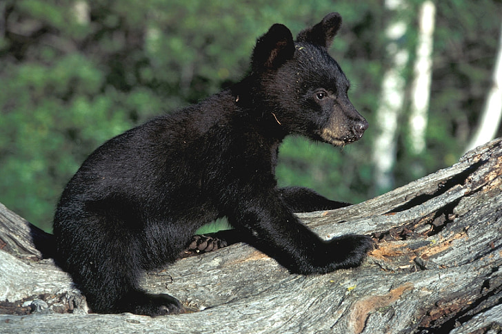
A biologist is studying black bears. In particular, what distribution best fits the weight (in ounces) of newborn black bear cubs? Their sample data contains 10 observations, \(x_1, x_2, \ldots , x_{10}\), corresponding the birth weight of 10 randomly selected black bear cubs.
Run the code cell below to “secretly” generate values for parameters that we store in mu.cub and sigma.cub.
A data frame called cub is created that has one variable, wt that has the sample birth weight data.
The command set.seed(113) will seed the randomization so we have the same parameter values and sample every time we run it.
Do not view the values of mu.cub or sigma.cub for now. Keep them secret for now!
set.seed(113) # fix randomizationmu.cub <-sample(seq(8.6, 9.8, 0.1), size=1) # set value of musigma.cub <-sample(seq(0.9, 1.3, 0.05), size=1) # set value of sigmapicked <-rnorm(10, mu.cub, sigma.cub) # pick a random sample n=10cub <-data.frame(wt = picked) # save sample to the cub data frameround(cub$wt, 2) # print sample to screen
Our goal is to find the “best” description of the distribution of all black bear cub birth weights. The interpretation of “best” depends on the context of the question and can mean different things to different statisticians.
Question 1
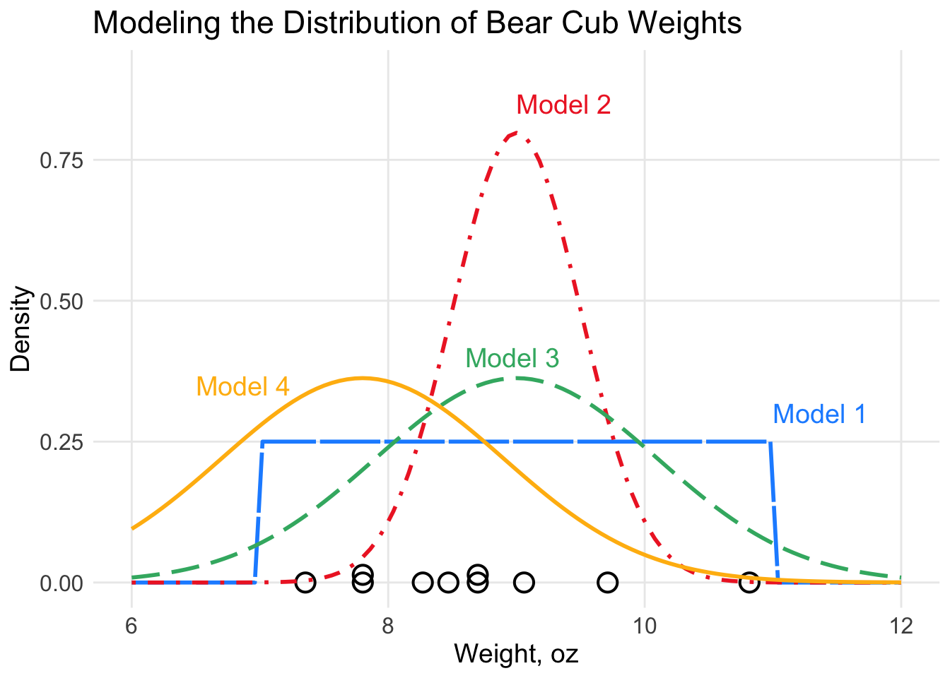
The figure below shows a dot plot of the selected sample (size \(n=10\)) of cub birth weights along with the plots of 4 different models we could choose for our data. Answer the questions based on plot figure below.
Figure 15.1: Comparing Models for Bear Cub Weights
Question 1a
Which of the models labeled 1-4 in the plot above do you believe best fits the sample data cub birth weights?
Solution to Question 1a
Question 1b
What type of continuous distribution best matches the graph you selected? Explain why in terms of birth weights of black bear cubs this distribution is reasonable and makes practical sense.
Using the sample of birth weights cub$wt, give estimates for each of the parameter(s) in the distribution you identified in Question 1b.
Solution to Question 1c
# be sure you have already run the first code cell and
# stored sample weights to variable `wt` in data frame `cub`
Based on your code above, what are the values of the parameters of the distribution in Question 1b?
Identifying Key Properties for Our Model
Let \(X\) be a random variable with pdf \(f(x; \theta_1, \theta_2, \ \ldots \theta_k)\) that depends on parameters \(\theta_1, \theta_2, \ldots , \theta_k\). If we independently pick random variables \(X_1, X_2, \ldots X_n\) from population \(X\), we can determine the values of \(\theta_1, \theta_2, \ldots , \theta_k\) that best fit the data in the following sense:
The mean \(\mu_X = E(X)\) of the population \(X\) equals the sample mean, \(\bar{x}\).
The variance \(\sigma^2_X = \mbox{Var}(X)\) of the population equals the variance of the sample, \(s^2\).
The skewness of the population equals the skewness of the sample.
The “peakiness” (kurtosis) of the population equals the “peakiness” of the sample.
\(\ldots\) and so on.
For example, in the birth weight of black bear cubs example, we assumed the population of birth weights \(X\) is normally distributed. Normal distributions are determined by two parameters, \(\mu\) and \(\sigma\).
The random sample has \(\bar{x} = 8.668\). We estimate \(E(X) = \mu=\bar{x} = 8.668\).
The random sample has \(s^2 = 1.032\). We estimate \(\mbox{Var(X)} = \sigma^2=s^2=1.032\).
We find values of the parameters so the properties of random variable \(X\) are equal to corresponding statistics from our sample.
Theoretical Moments
Let \(X\) be a random variable with pdf \(f(x)\). For a positive integer \(k\), the kth theoretical moment of \(X\) is \(\color{dodgerblue}{\mu_k = E \left( X^k \right) }\).
The fourth moment is \(\color{mediumpurple}{\mu_4 = E \left( X^4 \right) }\).
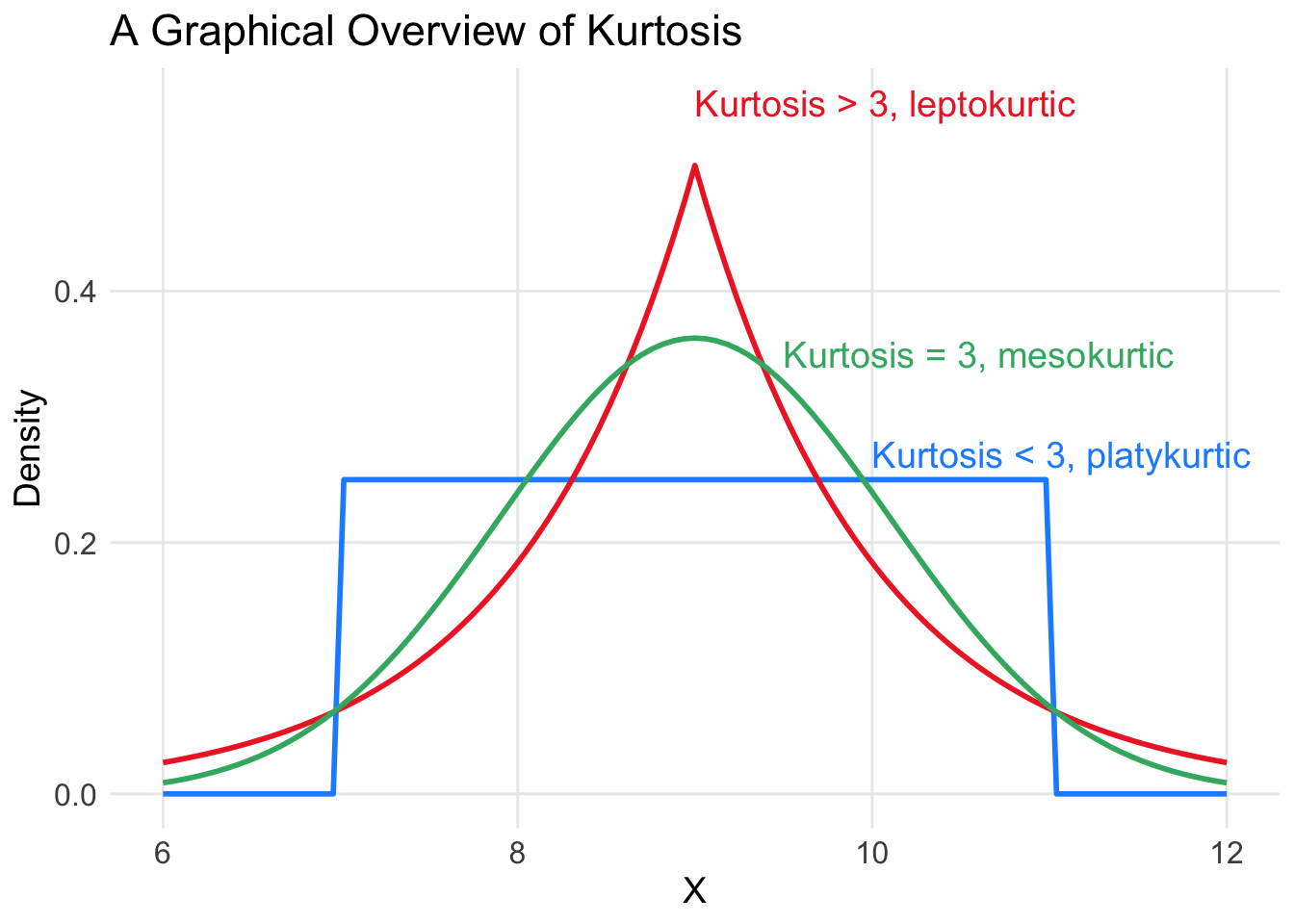
\(\mu_4\) is related to the kurtosis of \(X\) which is defined as \(E \big( (X-\mu_1)^4 \big)\).
Informally, the kurtosis measures how “peaky” or flat the distribution is.
Figure 16.1: A Graphical Overview of Kurtosis
Sample Moments
For a sample \(X_1=x_1, X_2=x_2, \ldots , X_n=x_n\), we can calculate the corresponding sample moments.
The first sample moment is \(\displaystyle M_1 = \frac{1}{n} \sum_{i=1}^n x_i\).
The second sample moment is \(\displaystyle M_2 = \frac{1}{n} \sum_{i=1}^n x_i^2\).
The kth sample moment is \(\color{dodgerblue}{\displaystyle M_k = \frac{1}{n} \sum_{i=1}^n x_i^k }\).
Note
We use Latin letters \(\color{dodgerblue}{M_k}\) to denote sample moments and Greek letters \(\color{tomato}{\mu_k}\) to denote theoretical moments for the population.
Applying integration methods, we can evaluate the integrals in Question 2a to get the following expressions for the first and second theoretical moments.
What integration methods do you believe will be useful to integrate the formulas in Question 2a? Explain in words how you could evaluate each of the integrals.
Time permitting: Refresh your integration skills by verifying the formulas for \(\mu_1\) and \(\mu_2\).
Solution to Question 2b
Question 2c
Let \(X_1=3\), \(X_2=4\), \(X_3 = 5\), and \(X_4 = 8\) be a random sample from the random variable \(X\) from Question 2. Find the first and second sample moments.
Solution to Question 2c
Defining the Method of Moments Estimate
Let \(X\) be a random variable with pdf \(f(x; \theta_1, \theta_2, \ldots, \theta_k)\) and let \(X_1\), \(X_2\), \(\ldots\), \(X_n\) be a random sample.
Compute sample moments \(M_1, M_2, \ldots , M_k\) based on the sample data.
Find formulas for the the theoretical moments \(\mu_1, \mu_2, \ldots , \mu_k\).
The formulas for the theoretical moments will depend on the parameters \(\theta_1, \theta_2, \ldots, \theta_k\).
The method of moments (MOM) estimate is obtained by solving the system:
Note: If \(X\) is a discrete random variable, change the integrals to summations.
We need to set up as many equations as the number of parameters in the pdf for random variable \(X\).
If the distribution has one parameter, we will only need to solve one equation \(\mu_1 = M_1\).
If the distribution has two parameters, we will need to solve a system fo two equations involving the first and second moments.
We will not encounter any distribution with more than two parameters this semester, though this method can be extended to distributions with more 3 or more parameters.
Practice
Question 3
Let \(X\) be a random variable from Question 2 with pdf \(\displaystyle f(x; \lambda, \delta)=\lambda e^{-\lambda(x-\delta)}\) for \(x > \delta\) with parameters \(\lambda, \delta >0\). The first and second theoretical moments (see Question 2a and Question 2b) are
Let \(X_1=3\), \(X_2=4\), \(X_3 = 5\), and \(X_4 = 8\) be a random sample from \(X\). Find \(\hat{\lambda}_{\rm{MoM}}\) and \(\hat{\delta}_{\rm{MoM}}\), the MoM estimates for parameters \(\lambda\) and \(\delta\). Hint: Use the sample moments from Question 2c.
Solution to Question 3
Question 4
Let \(X_1=1, X_2=3, X_3=7, X_4=10\) be four numbers picked at random from a continuous uniform distribution on \(\lbrack \alpha , \beta \rbrack\). Find the MoM estimates of \(\alpha\) and \(\beta\).
Tip
You do not need to evaluate any integrals to find expressions for \(\mu_1\) and \(\mu_2\). Recall if \(X\) is a continuous uniform distribtion, we have
\(\mu_2 \ne \mbox{Var}(X)\). However, you can derive a formula for \(\mu_2 = E(X^2)\) from formulas for both \(\mbox{Var}(X)\) and \(E(X)\).
Solution to Question 4
Question 5
Let \(X_1=1, X_2=3, X_3=3, X_4=2\) be four values picked at random from a binomial distribution \(X \sim \mbox{Binom}(n,p)\). Find the MoM estimates of \(n\) and \(p\).
Solution to Question 5
Question 6
Let \(X_1=x_1, X_2=x_2, \ldots X_n=x_n\) denote a random sample size \(n\) from the continuous uniform distribution on \(\lbrack \alpha , \beta \rbrack\).
Question 6a
Derive the following general formulas for the MoM estimates of \(\alpha\) and \(\beta\):
where \(M_1=\bar{x} = \frac{1}{n}\sum_{i=1}^n x_i\) and \(M_2= \frac{1}{n} \sum_{i=1}^n x_i^2\) denote the first and second sample moments, respectively. Find the MoM estimates of \(\alpha\) and \(\beta\).
Solution to Question 6a
Question 6b
Verify your solution to Question 4 using the formulas for the MoM estimates for \(\alpha\) and \(\beta\) in Question 6a.
Complete and run the partially completed R code cell below.
Solution to Question 6b
Replace each of the two ?? in the code cell below with appropriate code. Then run the completed code to check the MoM estimates for \(\hat{\alpha}_{\rm{MoM}}\) and \(\hat{\beta}_{\rm{MoM}}\) obtained Question 4.
x.unif <-c(1, 3, 7, 10) # sample from question 4n <-length(x.unif) # length of samplem1 <-sum(x.unif)/n # first sample momentm2 <-sum(x.unif^2)/n # second sample momentalpha.hat <- ?? # enter formula for MoM estimate for alphabeta.hat <- ?? # enter formula for MoM estimate for beta# print results to screenalpha.hatbeta.hat
Question 7
The code below generates sampling distributions for MoM estimates for the parameters \(\alpha\) and \(\beta\) for random variable \(X \sim \mbox{Unif}(\alpha, \beta)\) using sample size \(n=4\).
A total of 1,000 random samples each of size \(n\) are generated in the for loop.
The distribution of \(\hat{\alpha}_{\rm{MoM}}\) values are stored in the vector mom.alpha.
The distribution of \(\hat{\beta}_{\rm{MoM}}\) values are stored in the vector mom.beta.
############################## do not edit# run the code cell as is#############################n <-4# sample sizemom.alpha <-numeric(1000)mom.beta <-numeric(1000)for (i in1:1000){ x.temp <-runif(n, 0, 11) # generate random sample m1 <-sum(x.temp)/n # first sample moment m2 <-sum(x.temp^2)/n # second sample moment k <-sqrt(3) *sqrt(m2 - m1^2) # compute sqrt(3)*(m2 - m1^2) mom.alpha[i] <- m1 - k # enter formula for MoM estimate for alpha mom.beta[i] <- m1 + k # enter formula for MoM estimate for beta}
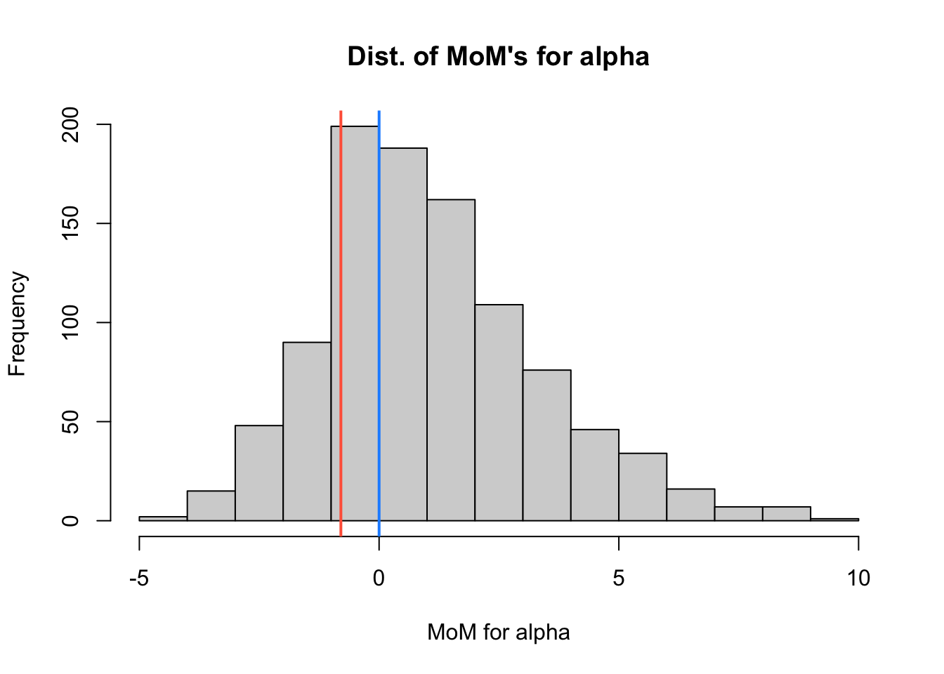
The distribution of \(\hat{\alpha}_{\rm{MoM}}\) values generated by the code above is plotted in the histogram below.
A blue vertical line is drawn at the actual value of \(\color{dodgerblue}{\alpha=0}\).
A red vertical line is drawn at the value of \(\color{tomato}{\hat{\alpha}_{\rm{MoM}}=-0.797}\) we found for the sample in Question 4.
############################## do not edit# run the code cell as is#############################hist(mom.alpha, breaks =20,xlab ="MoM for alpha",main ="Dist. of MoM's for alpha")abline(v =0, col ="dodgerblue", lwd =2) # plot at actual value of alphaabline(v =-0.797, col ="tomato", lwd =2) # plot at estimated value of alpha
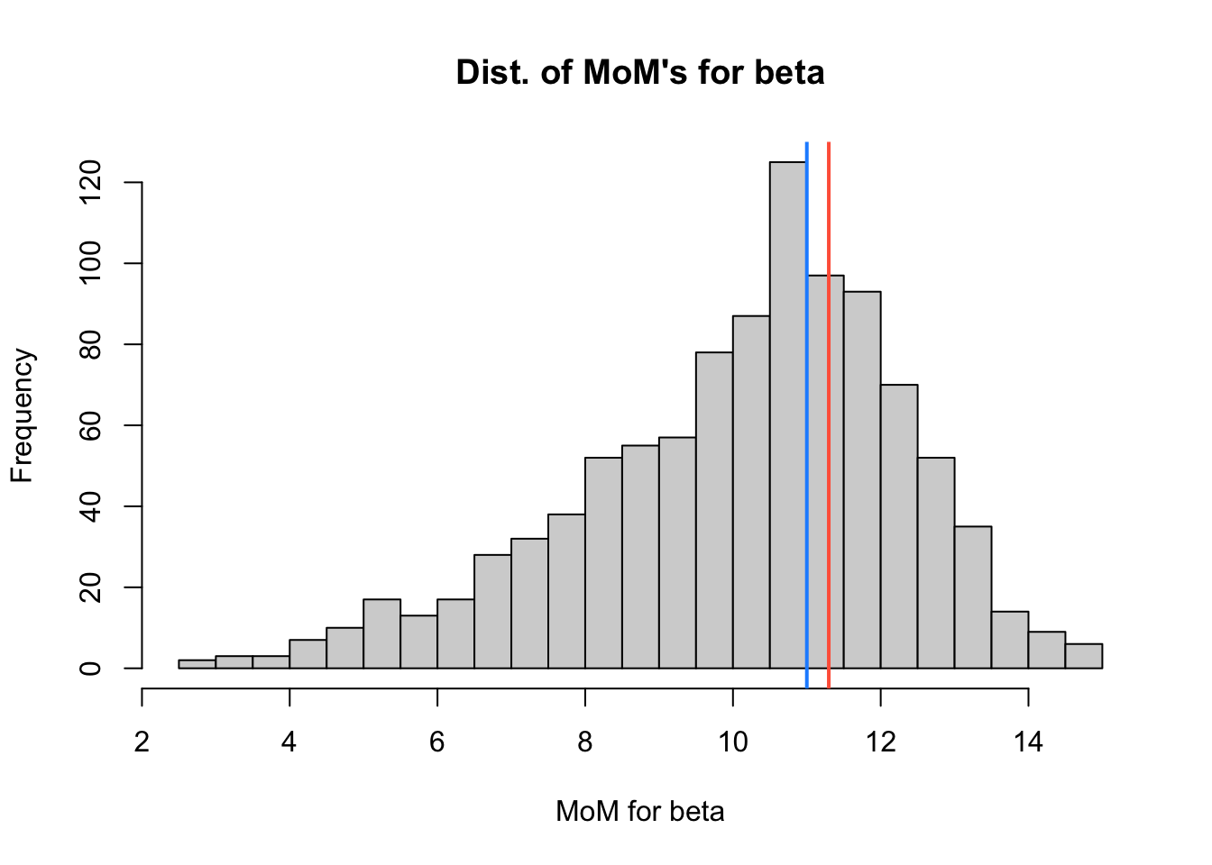
The distribution of \(\hat{\beta}_{\rm{MoM}}\) values generated by the code above is plotted in the histogram below.
A blue vertical line is drawn at the actual value of \(\color{dodgerblue}{\beta=11}\).
A red vertical line is drawn at the value of \(\color{tomato}{\hat{\beta}_{\rm{MoM}}=11.297}\) we found for the sample in Question 4.
############################## do not edit# run the code cell as is#############################hist(mom.beta, breaks =20,xlab ="MoM for beta",main ="Dist. of MoM's for beta")abline(v =11, col ="dodgerblue", lwd =2) # plot at actual value of betaabline(v =11.297, col ="tomato", lwd =2) # plot at estimated value of alpha
Question 7a
Based on inspecting the the sampling distributions plotted for \(\hat{\alpha}_{\rm{MoM}}\) and \(\hat{\beta}_{\rm{MoM}}\) in Question 7:
Do you believe the MoM estimator for \(\alpha\) is biased? Explain why or why not.
Do you believe the MoM estimator for \(\beta\) is biased? Explain why or why not.
Base your answers on the distribution of all estimates, not just the red vertical lines corresponding to the sample from Question 4.
Solution to Question 7a
Question 7b
Check your answers in Question 7a more carefully using the MoM estimates stored in mom.alpha and mom.beta.
Hint: Recall an estimator \(\hat{\theta}\) is unbiased if \(E(\hat{\theta}) = \theta\).
Solution to Question 7b
# check whether or not each estimator is biased
Question 7c
Which estimator, \(\hat{\alpha}_{\rm{MoM}}\) or \(\hat{\beta}_{\rm{MoM}}\), is more precise?
Hint: Recall the precision of an estimator \(\hat{\theta}\) is often measured by \(\mbox{Var}(\hat{\theta}) = \theta\).
Hint: Use R code and the MoM estimates stored in mom.alpha and mom.beta.
Solution to Question 7c
# check which estimator is more precise
Question 7d
Adjust the sample size in the first line in the first code cell below to investigate what happens to the distributions of estimators \(\hat{\alpha}_{\rm{MoM}}\) and \(\hat{\beta}_{\rm{MoM}}\). In particular, as \(n\) gets larger and larger:
Does each estimator seem to get more, less, or no change in bias?
Does each estimator get more, less, or no change in variability?
Does the shape of each distribution change?
Solution to Question 7d
Experiment with different sample sizes, \(n\).
######################## adjust sample size#######################n <-4# sample size###################################### do not edit the rest of the code#####################################mom.alpha <-numeric(1000)mom.beta <-numeric(1000)for (i in1:1000){ x.temp <-runif(n, 0, 11) # generate random sample m1 <-sum(x.temp)/n # first sample moment m2 <-sum(x.temp^2)/n # second sample moment k <-sqrt(3) *sqrt(m2 - m1^2) # compute sqrt(3)*(m2 - m1^2) mom.alpha[i] <- m1 - k # enter formula for MoM estimate for alpha mom.beta[i] <- m1 + k # enter formula for MoM estimate for beta}
########################################### sampling distribution for MoM of alpha# do not edit cell, just run##########################################hist(mom.alpha, breaks =20,xlab ="MoM for alpha",main ="Dist. of MoM's for alpha")abline(v =0, col ="dodgerblue", lwd =2) # plot at actual value of alpha
########################################### sampling distribution for MoM of beta# do not edit cell, just run##########################################hist(mom.beta, breaks =20,xlab ="MoM for beta",main ="Dist. of MoM's for beta")abline(v =11, col ="dodgerblue", lwd =2) # plot at actual value of beta
Exploring Bias of Each Estimator
As \(n\) gets larger, does each estimator seem to get more, less, or no change in bias?
# check for change to bias
Exploring Variability of Estimators
As \(n\) gets larger, does each estimator get more, less, or no change in variability?
# check for change in variability
Exploring the Shape of Sampling Distributions
Does the shape of each distribution change as \(n\) gets larger?

