hits <- read.csv("https://raw.githubusercontent.com/CU-Denver-MathStats-OER/Statistical-Theory/main/Data/spotify-hits.csv")2.2: Introduction to Random Variables
![]()
Randomness in a Music Playlist
Importing the Spotify Hits Data Set
The data set spotify-hits.csv1 is stored online and contains audio statistics of the top 2000 tracks on Spotify from 2000-2019. The data is stored in a comma separated file (csv). We can use the function read.csv() to import the csv file into an R data frame we call hits.
Cleaning the Music Data Set
In the code cell below:
- We convert
artist,song, andgenreto categorical variables using thefactor()function. - Extract the variables
artist,song,tempoandgenre(ignoring the rest). - Print the first 6 rows to screen to get a glimpse of the resulting data frame.
hits$artist <- factor(hits$artist)  # artist is categorical
hits$song <- factor(hits$song)  # song is categorical
hits$genre <- factor(hits$genre)  # genre is categorical
hits <- hits[,c("artist", "song", "tempo", "genre")]
head(hits)  # display first 6 rows of data frame
artist song tempo genre
1 Britney Spears Oops!...I Did It Again 95.053 pop
2 blink-182 All The Small Things 148.726 rock, pop
3 Faith Hill Breathe 136.859 pop, country
4 Bon Jovi It's My Life 119.992 rock, metal
5 *NSYNC Bye Bye Bye 172.656 pop
6 Sisqo Thong Song 121.549 hip hop, pop, R&BQuestion 1
Explore the data set hits. For example:
- How many observations are in the data set?
- Which artist had the most hits?
- What is the mean tempo?
- Create a plot to display the distribution of tempo scores.
- What genre occurs most frequently?
Solution to Question 1
Creating a Random Playlist
To create a random playlist of five songs from the hits library of songs, we can run the code cell below.
- The
sample()function below has three inputs:- The “population” we will be sampling from.
nrow(hits)returns the value 2000, the total number of observations (rows) in the data frame.
- The
sizeis the number of observations we will select. - The
replace =TRUEoptions means we sample with replacement. Each time we pick a song, we place it back into the population and can select it in our playlist again. - Run
?samplefor more information.
- The “population” we will be sampling from.
- We save the selected songs to the object called
playlist. - We print the list of songs in
playlistto the screen
# index contains the 5 randomly selected songs
index <- sample(nrow(hits), size=5, replace = TRUE)
playlist <- hits[index,]  # save each song from index to a playlist
head(playlist)  # print the playlist
artist song tempo
1072 Drake Over 100.093
193 Gabrielle Out Of Reach 182.862
119 iio Rapture (feat.Nadia Ali) 123.943
1585 Jack Ü Where Are Ü Now (with Justin Bieber) 139.432
1131 Cobra Starship You Make Me Feel... (feat. Sabi) 131.959
genre
1072 hip hop, pop, R&B
193 pop, R&B
119 Dance/Electronic
1585 pop, Dance/Electronic
1131 pop, Dance/ElectronicRandom Variables
How likely is it that none of the songs are classified in the genre “pop”? How likely is it that at most three songs are classified in the genre “pop”?
How can we connect these questions about our data to the concepts of sample spaces and events to answer these question? The link can be made using random variables!
Definition of a Random Variable
A random variable is a function that maps each outcome \(\omega\) in the sample space \(\Omega\) to a real number \(X(\omega)\).
\[ X: \Omega \to \mathbb{R} \]
In the music playlist example, each playlist is a different outcome in the sample space. There are a total of \(2000^5 = 3.2 \times 10^{16}\) possible playlists in the sample space.
- We can define random variable \(X\) to be the number of songs in the playlist from the pop genre.
- For example, we could randomly select 5 songs with genres \(\omega =\) (hip hop, country, pop, rock, pop)
- Random variable \(X\) is \(X(\omega) = 2\) since there are 2 pop songs in the playlist.
- The set of possible values for \(X\) is the discrete set \(\left\{ 0, 1, 2, 3, 4, 5 \right\}\).
Counting Pop Songs
One potential tricky issue with song genre is many songs are classified in multiple genres. The blink-182 song All The Small Things is in both the pop and rock genres. To simplify the analysis here, we will count songs that are only classified in pop genre (and no other genres). We will not count All The Small Things as a pop song since it is also classified as rock.
sum(hits$genre == "pop") # counts number of songs classified as only pop[1] 428- The
hitsdata frame contains 428 pop songs. - The proportion of all songs that are pop songs is \(\frac{428}{2000} = 0.214\) or \(21.4\%\).
Question 2
If \(21.4\%\) of all the songs are classified solely in the genre pop:
- Compute \(P(X=0)\), the probability of picking (with replacement) a random playlist of 5 songs that contains no pop songs.
- Compute \(P(X=5)\), the probability of picking (with replacement) a random playlist of 5 songs all of which are pop songs.
You can use an R code cell to help with the calculation.
# P(X = 0)


# P(X=5)
Solution to Question 2
Distributions for Discrete Random Variables
If \(X\) is a discrete random variable, we define the probability function or probability distribution or probability mass function (pmf) for \(X\) by
\[\color{dodgerblue}{p(x) = P(X=x)}.\]
If \(X\) is a discrete random variable, we define the cumulative distribution function (cdf) as the function
\[\color{dodgerblue}{F(x)=P(X \leq x) = \sum_{k=\rm{min \ value}}^x p(k) }.\]
The PMF and CDF for the Number of Pop Songs
In the case of counting the number of pop songs in a 5 song playlist, we can organize the values of the pmf \(p(x)\) in a table.
| \(x\) | 0 | 1 | 2 | 3 | 4 | 5 |
|---|---|---|---|---|---|---|
| \(p(x)\) | 0.3000 | 0.4084 | 0.2224 | 0.0606 | 0.0082 | 0.0004 |
From the pmf table above, we have the corresponding cdf below.
| \(x\) | 0 | 1 | 2 | 3 | 4 | 5 |
|---|---|---|---|---|---|---|
| \(F(x)\) | 0.3000 | 0.7084 | 0.9308 | 0.9914 | 0.9996 | 1 |
Question 3
Interpret the practical meaning of \(p(3) = 0.0606\) and \(F(3) = 0.9914\).
Solution to Question 3
Question 4
What is the probability of picking a playlist with at least 3 pop songs?
Solution to Question 4
Plotting Distribution Functions
n <- 5  # set number of trials n
p <- 0.241  # prob of success in a trial
x <- 0:n  # vector from 0 to n=3

par(mfrow=c(1, 2))
plot(x, dbinom(x, size = n, prob = p),
     main = "Graph of pmf",
     xlab = "Number of Pop Songs",
     ylab = "p(x)")

plot(x, pbinom(x, size = n, prob = p),
     type="s",
     main = "Graph of cdf",
     xlab = "Number of Pop Songs",
     ylab = "F(x)")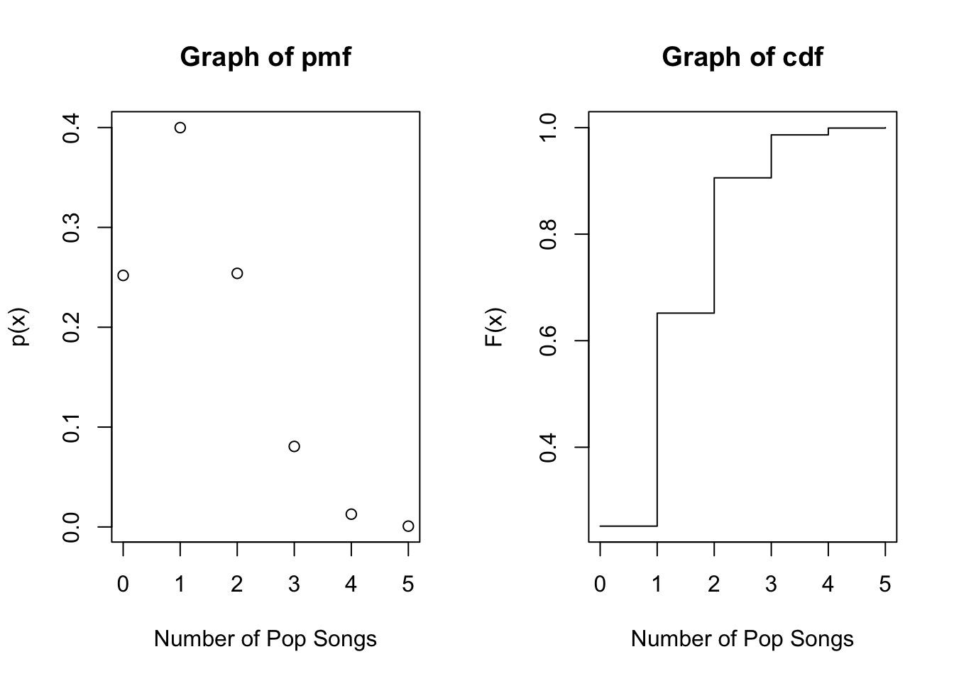
Question 5
Let \(X\) a discrete random variable with pmf and cdf denoted \(p(x)\) and \(F(x)\), respectively. Determine if each statement is True or False.
- \(0 \leq p(x) \leq 1\) for all \(x\).
- \(0 \leq F(x) \leq 1\) for all \(x\).
- \(\displaystyle \sum_{\rm{all}\ x} p(x) = 1\).
- \(\displaystyle \sum_{\rm{all}\ x} F(x) = 1\).
- \(\displaystyle \lim_{x \to \infty} p(x) = 1\).
- \(\displaystyle \lim_{x \to \infty} F(x) = 1\).
- The pmf must be a nondecreasing function.
- The cdf must be a nondecreasing function.
Solution to Question 5
List the properties (a)-(h) that are indeed TRUE.
Continuous Random Variables
Discrete random variables map outcomes in the sample space to integers. In many situations we would like to consider mapping outcomes to a continuous interval of values, not just integers. For example, what is the probability that randomly selected song has a tempo less than 82 beats per minute (BPM)?
- The sample space \(\Omega\) consists of the set of all songs in
hits. - \(X: \Omega \to \mathbb{R}\) where we map each selected song to its tempo (in BPM).
- The range is now a continuous interval of real numbers representing the tempos of all songs in
hits.
Using modern technology such as music sequencers tempo has become a very precise measurement. Tempo is an important characteristic in electronic dance music where accurate measurement of a tune’s BPM is important to DJ’s when mixing music.
summary(hits$tempo) Min. 1st Qu. Median Mean 3rd Qu. Max.
60.02 98.99 120.02 120.12 134.27 210.85 - From the summary above, we see tempo is a continuous measurement (it has decimal values) from a minimum of \(60.02\) BPM to a maximum \(210.85\) BPM.
Question 6
Below is a histogram representing the distribution of tempos for the 2000 songs in hits. Approximate the value of \(P(X < 85)\), the probability that a randomly selected songs has a tempo less than 85 BPM.
- Experiment with the number of breaks to improve the accuracy of your approximation!
# create a histogram
hist(hits$tempo,  # vector of tempo measurements
########################################################
# Student To-Do: Adjust breaks
########################################################
     breaks = 10,  # number of bin ranges to use
########################################################
     labels = TRUE,  # add count labels above each bar
     xlab = "Tempo (BPM)",   # x-axis label
     xaxt='n',  # turn off default x-axis ticks
     yaxt='n',  # turn off default y-axis ticks
     ylab = "Frequency",  # y-axis label
     ylim = c(0,650),  # sets window for y-axis
     main = "Distribution of Tempos",  # main label
     col = "steelblue")  # fill color of bars
axis(1, at = seq(60, 220, 10))  # set custom ticks on x-axis
axis(2, at = seq(0, 650, 50))  # set custom ticks on y-axis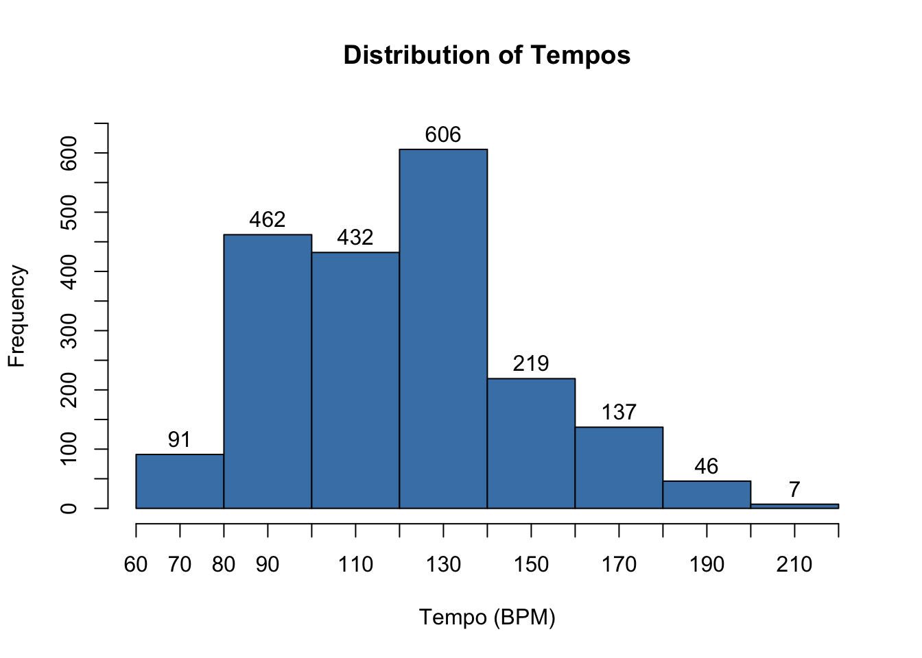
Solution to Question 6
Relative Frequency Histograms
Our initial frequency histogram of tempos in Question 6 measured the count or frequency of songs that fall in each bin of the histogram. A relative frequency histogram rescales the vertical axis to units proportion per unit of \(X\).
- We can create a relative frequency histogram by adding the option
freq = FALSEin thehist()function.
Question 7
Based on the relative frequency histogram below, approximate the value of \(P(X < 85)\), the probability that a randomly selected songs has a tempo less than 85 BPM.
The option
freq = FALSEis added to thehistcommand below. Run the code cell below and compare the result with the histogram above. What is different about the two histograms? What is similar? What are the units of the horizontal axis?Using the output from the code cell below, approximate \(P(X < 85)\). Hint: The area of each bar corresponds to the proportion of songs in
hitsthat are in the corresponding bin range of tempos.
# create a histogram
hist(hits$tempo,  # vector of tempo measurements
     freq = FALSE,
     breaks = 20,  # number of bin ranges to use
     labels = TRUE,  # add count labels above each bar
     xlab = "Tempo (BPM)",   # x-axis label
     xaxt='n',  # turn off default x-axis ticks
     yaxt='n',  # turn off default y-axis ticks
     ylab = "Relative Frequency",  # y-axis label
     ylim = c(0,0.025),  # sets window for y-axis
     main = "Distribution of Tempos",  # main label
     col = "steelblue")  # fill color of bars
axis(1, at = seq(60, 220, 10))  # set custom ticks on x-axis
axis(2, at = seq(0, 0.025, 0.005))  # set custom ticks on y-axis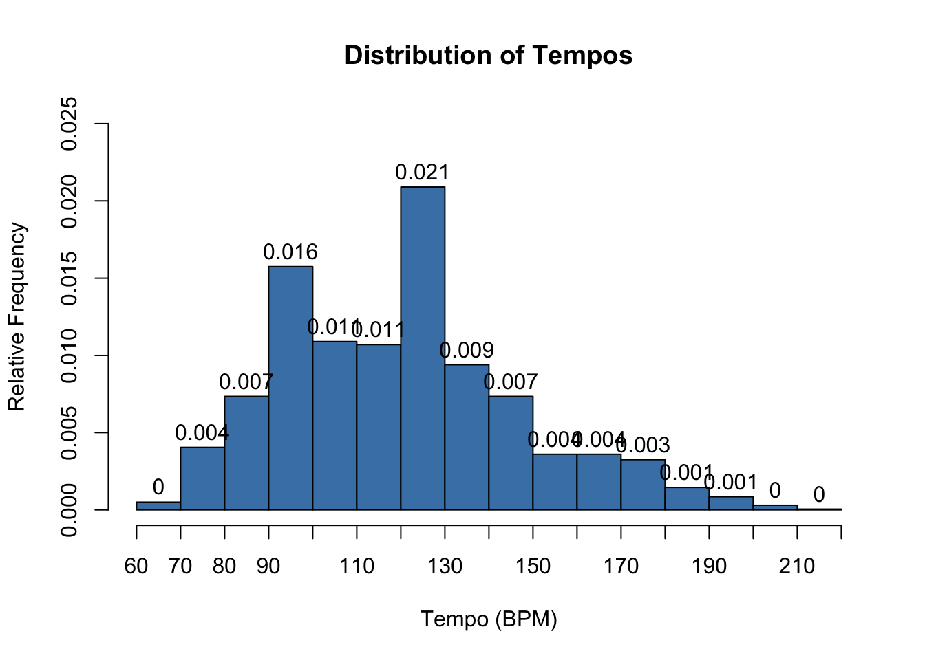
Solution to Question 7
Density Plots
A density plot can informally be considered as a relative frequency histogram where we choose incredibly small widths for each bin range. One way to create a density plot in R is to:
- First convert the values of a quantitative variable to densities with the
density()function.
- For more information, see density help documentation.
- Use the
plot()function to plot the densities.
- For more advanced density plots see https://r-graph-gallery.com/density-plot.html.
# approximate densities and then plot
plot(density(hits$tempo),  # convert to density and then plot
     ylab = "density (proportion per BPM)",  # vertical axis label
     xlab = "Tempo (in BPM)",  # horizontal axis label
     main = "Distribution of Song Tempos")  # main title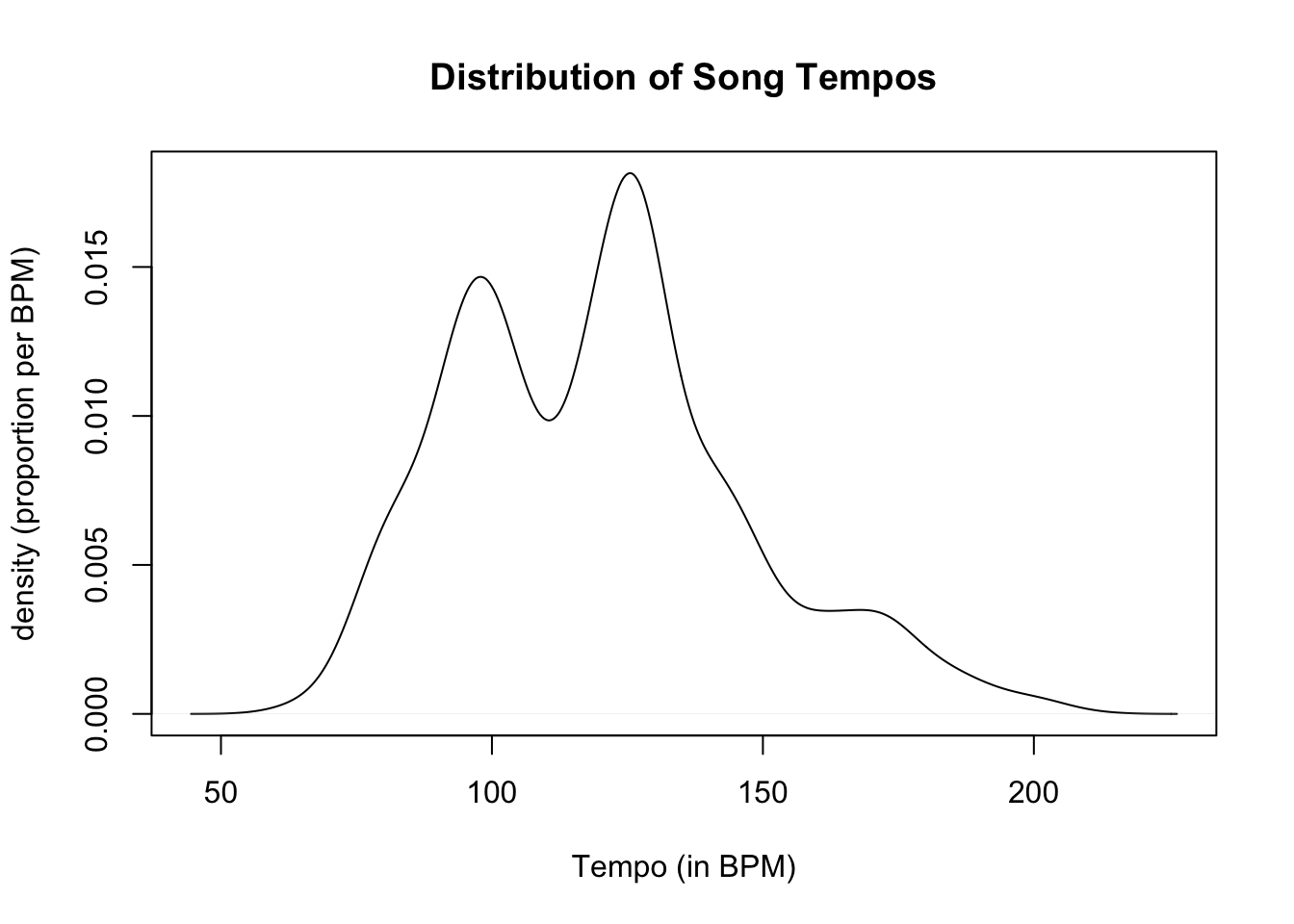
Reading a Density Plot
If we want to use a density plot compute \(P(X < 85)\), the probability that a random selected song in hits has a tempo less than 85 BPM:
- We approximate the AREA below the density curve over the interval from 0 to 85 BPM.
- If we have a theoretical model \(f(x)\) for the density, we can use definite integrals to compute these proportions!
- Run the code cell below to sketch an area corresponding to \(P(X<85)\). There is nothing to edit in the code cell.
###############################
# Area representing P(X < 85)
# Run code without editting
##############################
den <- density(hits$tempo)

plot(den,  # plot density of tempo
     ylab = "density (proportion per BPM)",  # vertical axis label
     xlab = "Tempo (in BPM)",  # horizontal axis label
     xaxt = 'n',  # turn off default x-axis ticks
     main = "Distribution of Song Tempos")  # main title


# Fill area from 0 to 85 BPM
value <- 85

polygon(c(den$x[den$x <= value ], value),
        c(den$y[den$x <= value ], 0),
        col = "slateblue1",
        border = 1)
axis(1, at = seq(0, value, value))  # set custom ticks on x-axis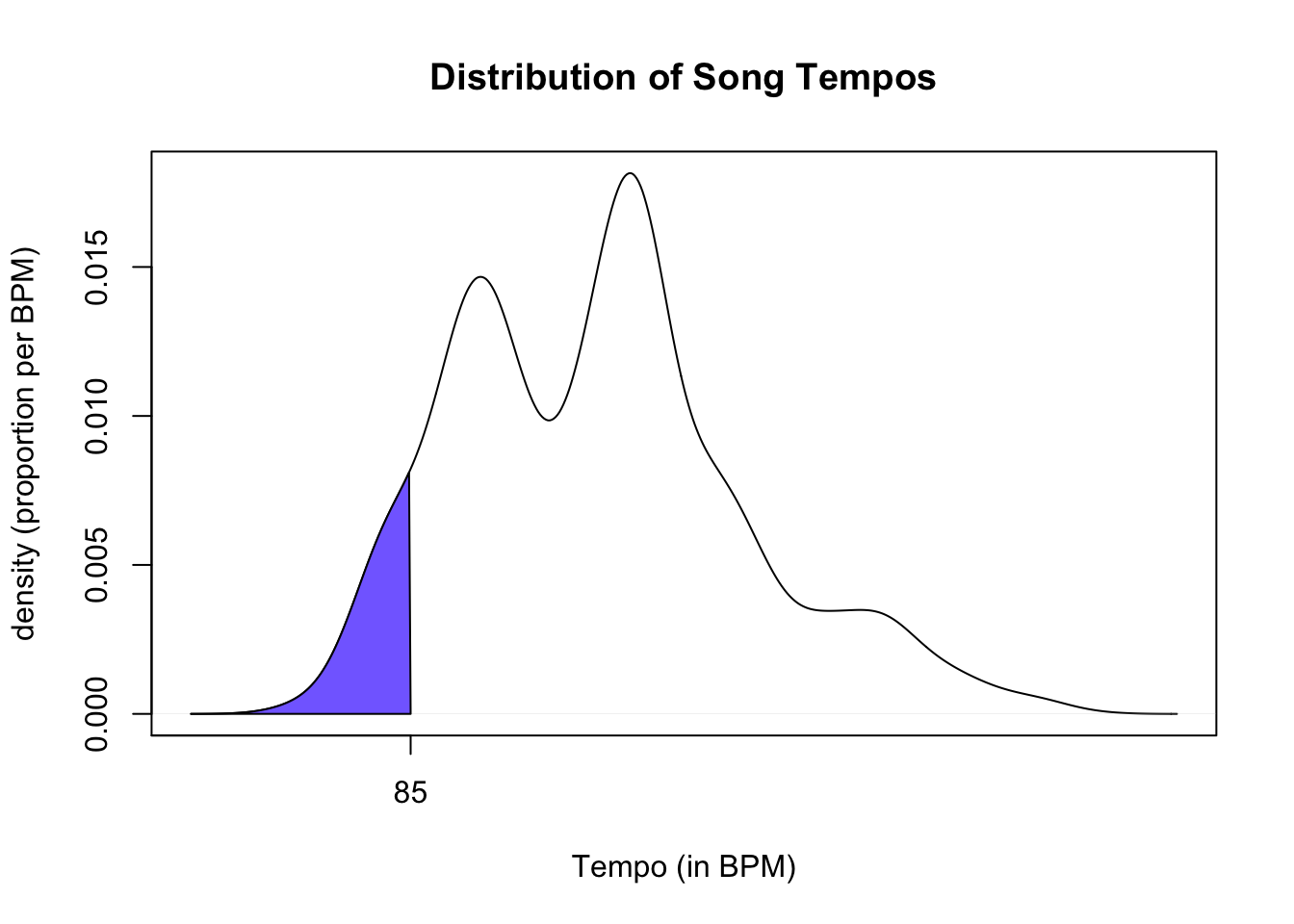
Continuous Probability Distributions
Probability Density Function (pdf)
If \(X\) is a continuous random variable, the probability density function (pdf), denoted \(f(x)\), satisfies the following properties:
- \(f(x) \geq 0\) for all \(x\),
- \(\displaystyle \int_{-\infty}^{\infty} f(x) = 1\), and
- \(\displaystyle P(a < x < b) = \int_a^b f(x) \, dx\)
Cumulative Distribution Function (cdf)
If \(X\) is a continuous random variable, the cumulative distribution function (cdf), denoted \(F(x)\), is
\[\color{dodgerblue}{F(x) = P(X < x) = \int_{-\infty}^x f(t) \, dt}.\]
Thus we have the important relations between a pdf and cdf of a continuous random variable X:
- The cdf \(F(x)\) is an antiderivative of the pdf \(f\).
- The pdf \(f(x)\) is the derivative of \(F(x)\).
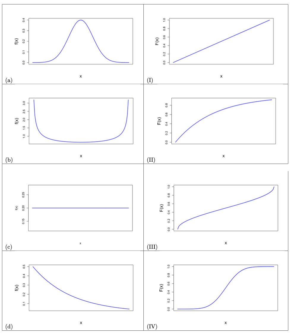
Question 8
The figure below contains 8 plots of either a probability density function or a cumulative distribution function of a continuous random variable. Match each probability density function shown in (a)-(d) with a corresponding graph of a cumulative distribution function (I)-(IV). Explain how you determined your answers.
Solution to Question 8
| Graph (a) | Graph (b) | Graph (c) | Graph (d) |
|---|---|---|---|
| ?? | ?? | ?? | ?? |
Properties of Continuous Random Variables
Question 9
Let \(X\) is a continuous random variable with pdf and cdf denoted \(f(x)\) and \(F(x)\), respectively. Determine if each statement is True or False.
- \(0 \leq f(x) \leq 1\) for all \(x\).
- \(0 \leq F(x) \leq 1\) for all \(x\).
- \(\displaystyle \int_{\infty}^{-\infty} f(x) \, dx= 1\).
- \(\displaystyle \int_{\infty}^{-\infty} F(x) \, dx = 1\).
- \(\displaystyle \lim_{x \to \infty} f(x) = 1\).
- \(\displaystyle \lim_{x \to \infty} F(x) = 1\).
- The pdf must be a nondecreasing function.
- The cdf must be a nondecreasing function.
Solution to Question 9
List the properties (a)-(h) that are indeed TRUE.
Question 10
The probability of a Lithium-ion battery failing at time \(x\) (in years) is given by the probability density function below.
\[f(x) = \left\{ \begin{array}{ll} \frac{1}{3}e^{-\frac{x}{3}} & x \geq 0 \\ 0 & \mbox{otherwise} \end{array} \right.\]
Question 10a
Compute the probability that a Lithium-ion battery lasts more than 2 years.
Solution to Question 10a
Question 10b
Interpret the meaning of \(P(X \leq 3)\) and \(P(X < 3)\).
Solution to Question 10b

Statistical Methods: Exploring the Uncertain by Adam Spiegler is licensed under a Creative Commons Attribution-NonCommercial-ShareAlike 4.0 International License.