4.3: Properties of Estimators

In this section, we continue our study of estimators of population parameters. An estimator, denoted \(\color{dodgerblue}{\hat{\theta}}\), is a formula or rule that we use to estimate the value of an unknown population parameter \(\theta\). For a single parameter \(\theta\), there are many (possibly infinite) different estimators \(\hat{\theta}\) from which to choose from. We have more deeply investigated two particularly useful methods: maximum likelihood estimates (MLE) and method of moments estimation.

We can think of different estimators, \(\hat{\theta}\), as different paths attempting to arrive at the same destination, the value of \(\theta\). Different statisticians might prefer different paths, which path is optimal? Sometimes different methods lead to the same result, and sometimes they differ. When they differ, how do we decide which estimate is best?

Question 1

Suppose our population parameter of interest is the center of a dart board. We use four different methods for throwing darts and the results of those four different methods are displayed in Figure 15.1.

Question 1a

Rank the results of the four dart methods in terms of accuracy, from most to least accurate. Explain your reasoning.

Solution to Question 1a

Question 1b

Rank the results of the four dart methods in terms of precision, from most to least precise. Explain your reasoning.

Solution to Question 1b

Question 1c

Rank the results of the four dart methods from best to worst overall. Explain your reasoning.

Solution to Question 1c

Question 1d

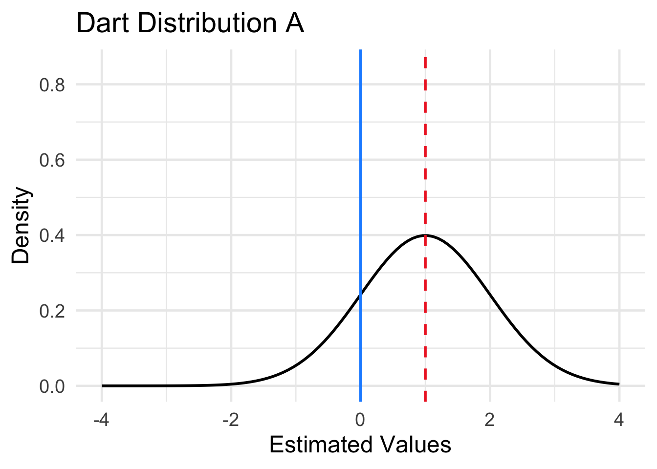
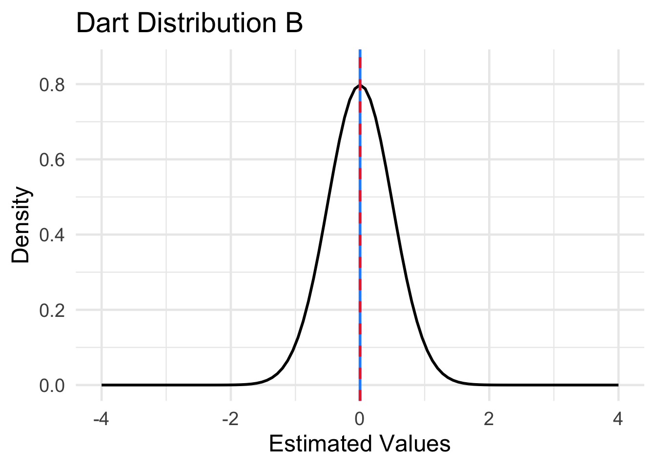
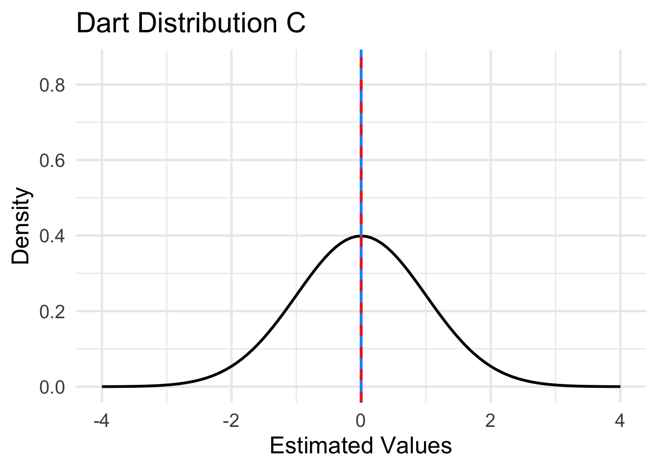
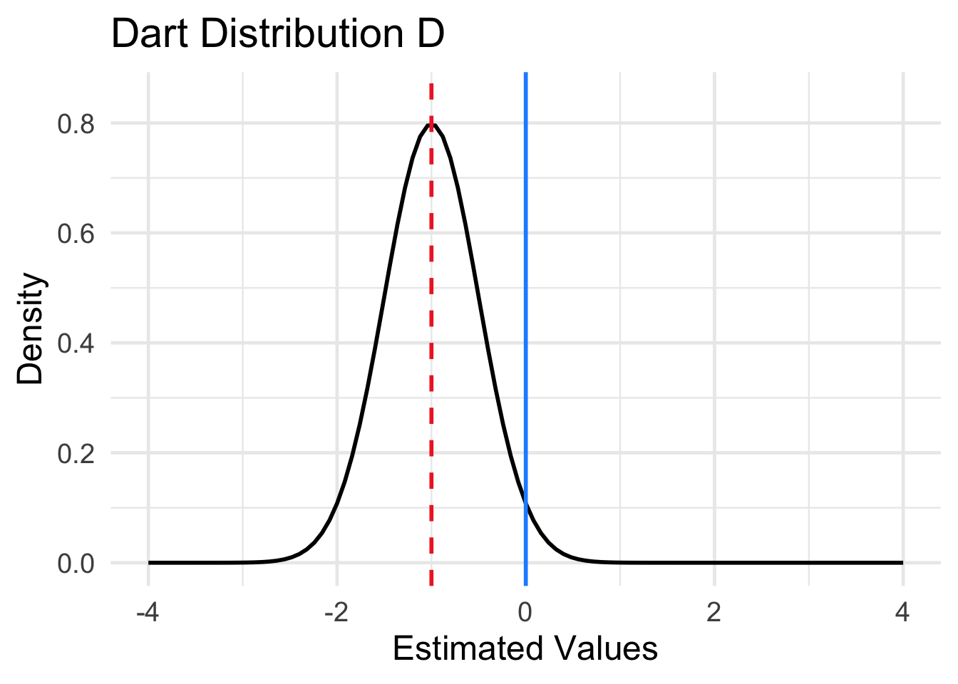
Four different sampling distributions of the results of the four dart throwing methods are plotted in Figure 15.2. The location of the population parameter (the center of the dart board) is indicated by the dashed red line. The mean of the sampling distribution is indicated by the solid blue vertical line. Match each of the distributions labeled A-D below to one of the four dart boards displayed in Question 1.

Solution to Question 1d

Dart Distribution A matches dart method ??.
Dart Distribution B matches dart method ??.
Dart Distribution C matches dart method ??.
Dart Distribution D matches dart method ??.

Comparing Estimators

At first glance, the question of which estimator is best may seem like a simple question.

The estimator that gives a value closest to the population parameter is best!

However, choosing the “best” estimator is not as straightforward as simply choosing the estimator that gives the value closest to the actual value. The parameters we are estimating are unknown values! We do not know where the center of the dart board is located. We cannot be certain which estimator leads to the closest estimate. Different samples will give different estimates even if we use the same formula for the estimator, and each estimate has some uncertainty due to sampling.

We might choose the “best” method but get “unlucky” by randomly selecting a biased sample.
We might choose a “bad” method but get “lucky” because we picked a good sample.

We can still choose a method that is more likely to give a better estimate (such as MLE) and/or minimizes the effect of the uncertainty due to sampling. Which properties are most important to consider depend on many factors. For example:

What is the parameter we are trying to estimate?
What is the shape of the distribution of the population?
Who are the statisticians/researchers? Different statisticians might have different goals.
How is the estimate going to assessed? For example, is precision or accuracy more important?

There are many properties of estimators worth considering when deciding between different estimators. In this section, we explore properties relating to accuracy (bias), precision (variability), and the mean squared error (MSE) which takes both bias and variability into consideration.

Question 2

Let \(X\) denote the diastolic blood pressure (in mm Hg) of a randomly selected woman from the Pima Indian Community. The Pima Indian Community is mostly located outside of Phoenix, Arizona. The data¹ used in this example is from the data frame Pima.tr in the MASS package.

If we suppose blood pressure is normally distributed, then we have \(X \sim N(\mu, \sigma)\). We would like to decide which estimator is best for the population mean \(\mu\). We pick a random sample of \(n=20\) women in the code cell below.

library(MASS)  # load MASS package to access data

set.seed(20)  # fix randomization of sample
x <- sample(Pima.tr$bp, size=20)  # pick a random sample of 20 blood pressures
x

 [1]  58  64  64  80  68  76  72 102  68  52  90  70  56  62  74  74  76  82  85
[20]  52

The random sample of diastolic blood pressure values is \[\mathbf{x} = (58, 64, 64, 80, 68, 76, 72, 102, 68, 52, 90, 70, 56, 62, 74, 74, 76, 82, 85, 52).\] Consider the following estimates for the population mean \(\mu\):

1. The sample mean: \(\hat{\mu}_1 = \bar{X} = \dfrac{\sum_{i=1}^n X_i}{n}\).

# 1. calculate sample mean
mu.hat1 <- mean(x)
mu.hat1

[1] 71.25

2. The sample median, denoted \(\hat{\mu}_2 = \mbox{median}\).

# 2. calculate sample median
mu.hat2 <- median(x)
mu.hat2

[1] 71

3. The mid-range of the sample, \(\hat{\mu}_3 = \dfrac{X_{\rm{max}} + X_{\rm{min}}}{2}\).

# 3. calculate sample mid range
mu.hat3 <- (max(x) + min(x)) / 2
mu.hat3

[1] 77

4. The sample trimmed (10%) mean, \(\bar{x}_{\rm{tr}(10)}\).

We exclude the smallest 10% of the values. The smallest 2 values, 52 and 52, are excluded.
We exclude the largest 10% of the values. The largest 2 values, 102 and 90, are excluded.
We compute the mean of the remaining 16 values.

# 4. calculate sample trimmed (10%) mean
mu.hat4 <- mean(x, trim = 0.1)
mu.hat4

[1] 70.5625

Question 2a

Which estimator (mean, median, mid-range, or trimmed mean) do you believe is best? Which estimator do you believe is the worst? Explain your reasoning.

Solution to Question 2a

Question 2b

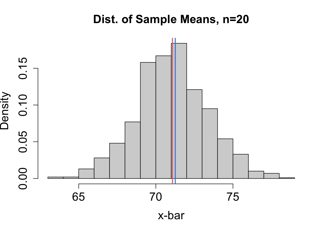
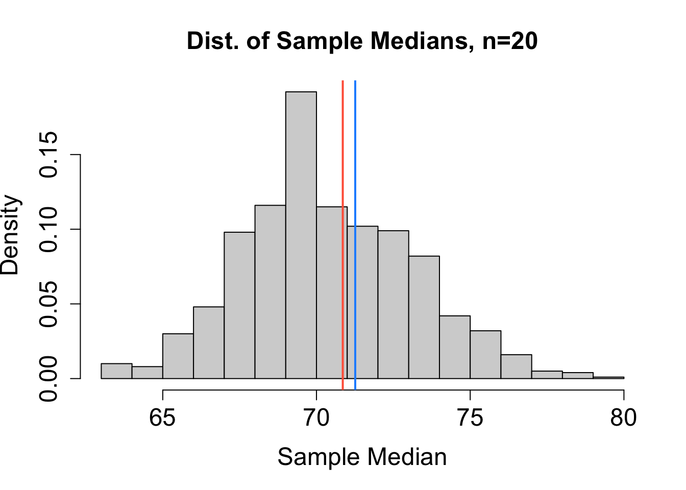
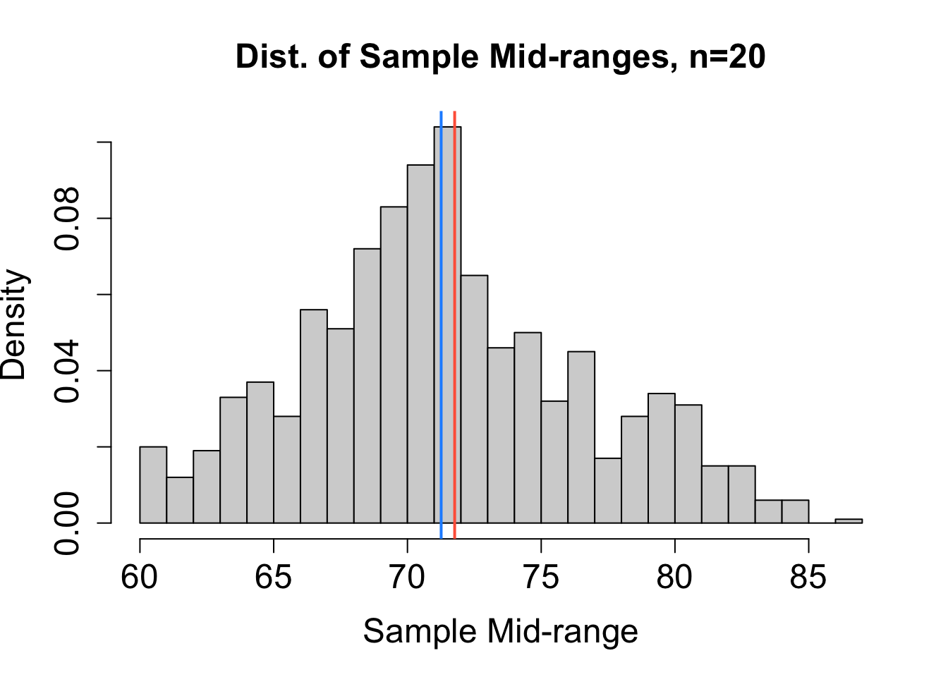
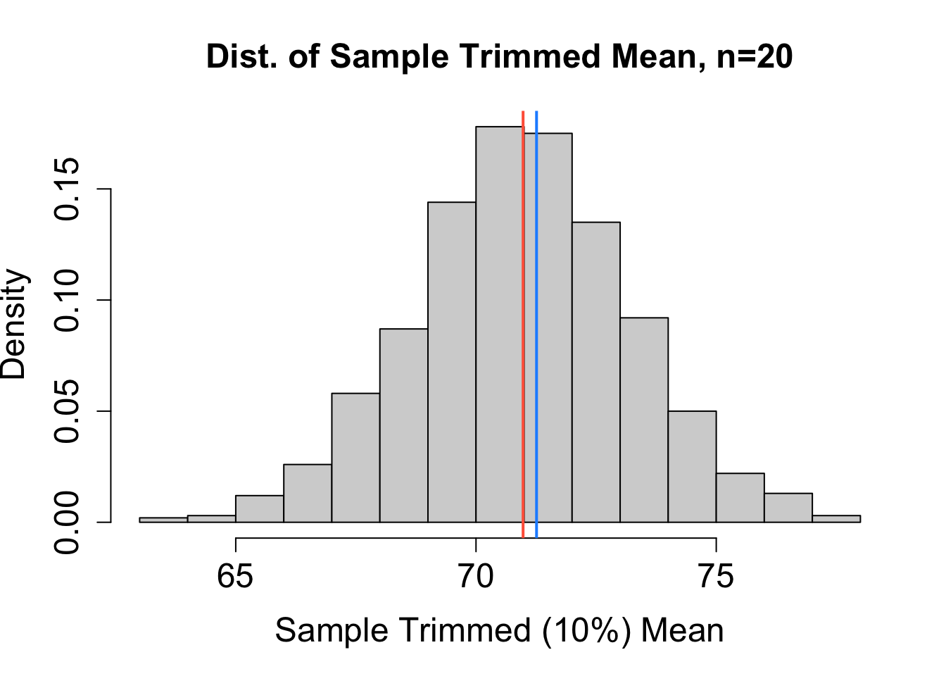
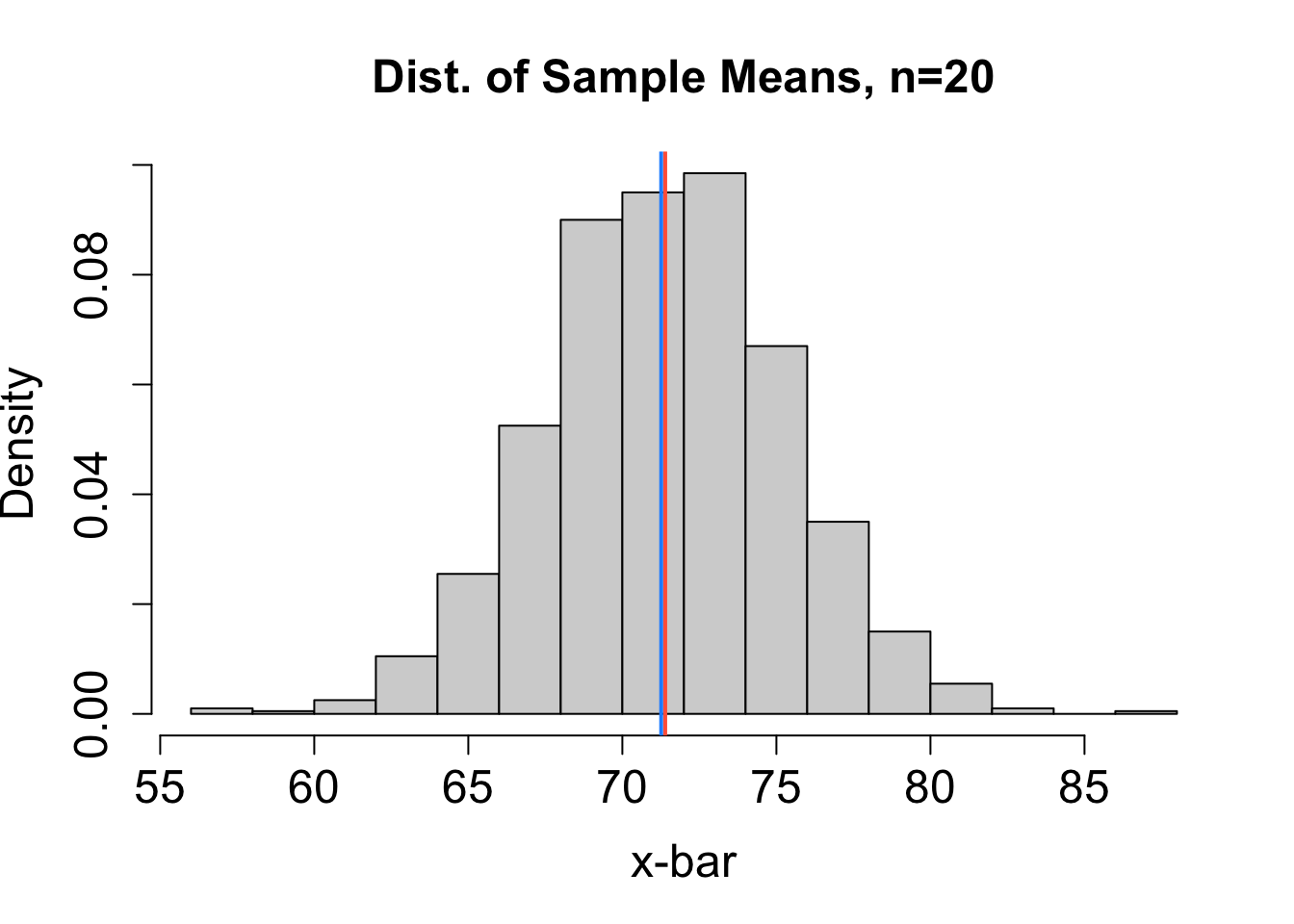
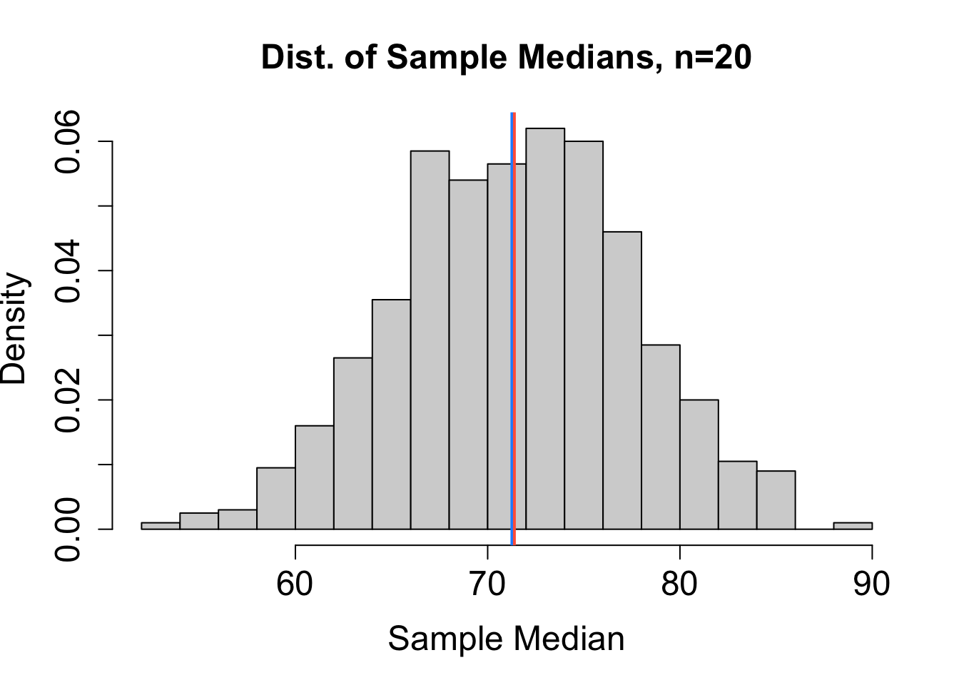
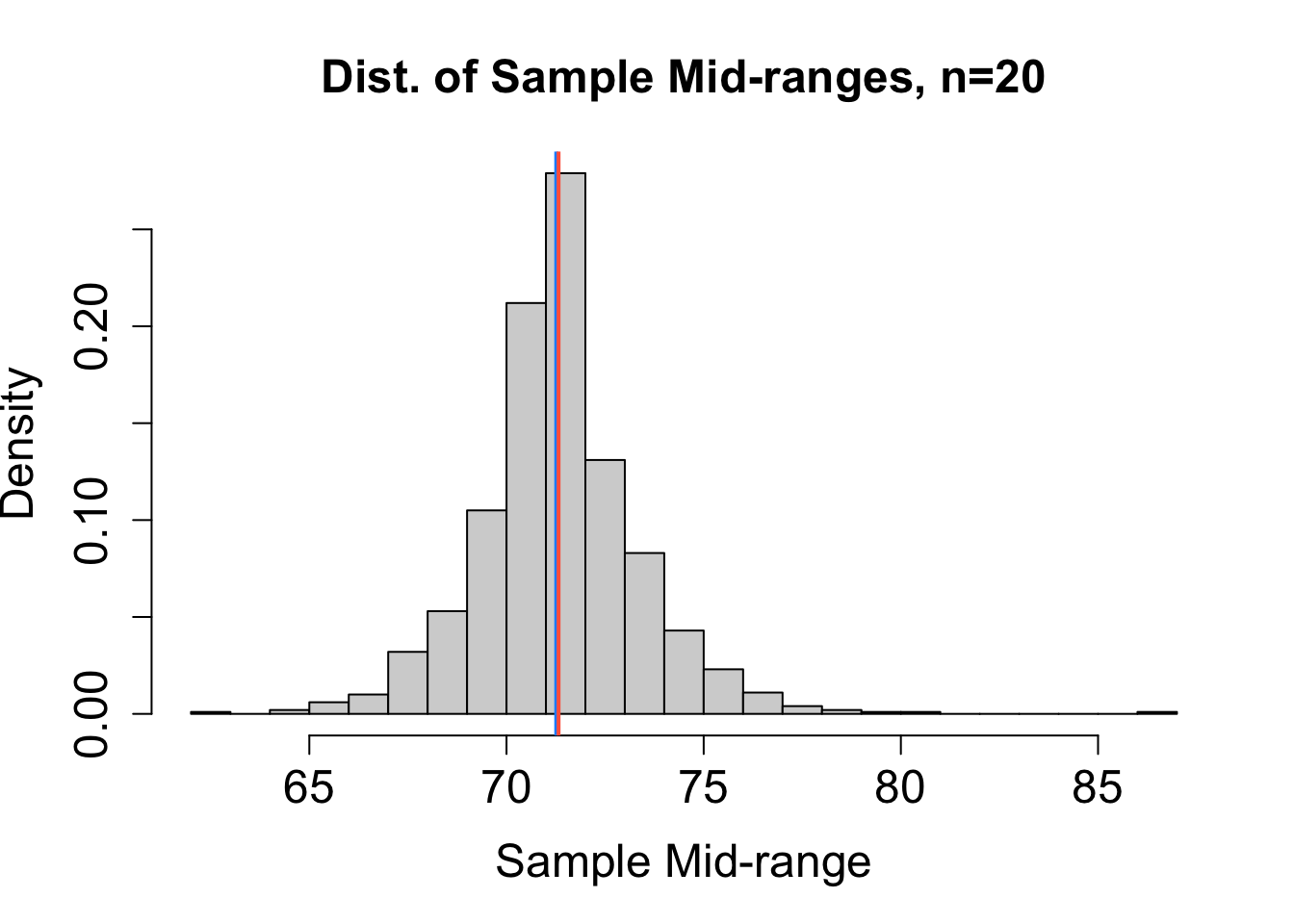
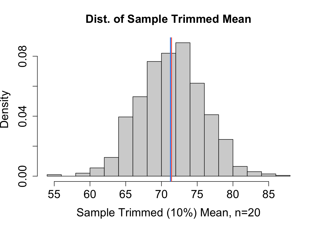
To help decide which estimator performs best, we can consider the sampling distribution of estimates obtained from many different random samples (each of size \(n=20\)) chosen independently from the same population. Based on the sampling distributions for \(\hat{\mu}_1\), \(\hat{\mu}_2\), \(\hat{\mu}_3\), and \(\hat{\mu}_4\) (mean, median, mid-range, and trimmed mean, respectively) in Figure 16.1, rank the four estimators from least to most bias and from most to least precise. The blue vertical line represents the actual value of \(\mu\). The red vertical line marks the expected value of the estimator. Explain your reasoning.

Solution to Question 2b

Question 2c

We still let \(X\) denote the diastolic blood pressure (in mm Hg) of a randomly selected woman from the Pima Indian Community. However, now we suppose blood pressure is uniformly distributed over the interval \(\lbrack 41.26, 101.26 \rbrack\). Although a uniform distribution would not make practical sense for blood pressure, we make this assumption in order to investigate how the shape of the population may affect which estimator works best.

Consider the sampling distribution of estimates obtained from many different random samples (each of size \(n=20\)) chosen independently from a uniformly distributed population. Based on the sampling distributions for \(\hat{\mu}_1\), \(\hat{\mu}_2\), \(\hat{\mu}_3\), and \(\hat{\mu}_4\) (mean, median, mid-range, and trimmed mean, respectively) in Figure 16.2, rank the four estimators again from least to most bias and from most to least precise. The blue vertical line represents the actual value of \(\mu\). The red vertical line marks the expected value of the estimator. Compare your updated rankings to those from Question 2b. Did your rankings change?

Solution to Question 2c

Bias of an Estimator

No matter what formula we choose as an estimator, the estimate we obtain will vary from sample to sample. We like an estimator to be, on average, equal to the parameter it is estimating. The bias of an estimator \(\hat{\theta }\) for parameter \(\theta\) is defined as the difference in the average (expected) value of the estimator and the parameter \(\theta\),

\[{\large \color{dodgerblue}{\boxed{ \mbox{Bias} = E(\hat{\theta}) - \theta.}}}\]

\(\hat{\theta}\) is an unbiased estimator if \(\color{dodgerblue}{\mbox{Bias} = E(\hat{\theta}) - \theta =0}\).
If the bias is positive, then on average \(\hat{\theta}\) gives an overestimate for \(\theta\).
If the bias is negative, then on average \(\hat{\theta}\) gives an underestimate for \(\theta\).

Estimates that are perfectly unbiased may be impossible or unreasonable at times. In practice, we are satisfied when estimates are approximately unbiased, or when the bias gets closer and closer to 0 as the sample size, \(n\), gets larger.

Question 3

Let \(X \sim \mbox{Binom}(n,p)\) with \(n\) known and parameter \(p\) unknown. Consider the following two estimators for parameter \(p\):

The usual sample proportion, \(\hat{p} = \frac{X}{n}\).
A modified proportion, \(\tilde{p} = \frac{X+2}{n+4}\). This is equivalent to adding 4 more trials to the sample, 2 of which are successes.

Tip

Use properties of expected value and recall these useful formulas for \(X \sim \mbox{Binom}(n,p)\),

\[E(X) = np \quad \mbox{and} \quad \mbox{Var}(X) = np(1-p).\]

Question 3a

Determine whether the estimator \(\hat{p} = \frac{X}{n}\) is biased or unbiased.

Solution to Question 3a

Question 3b

Determine whether the estimator \(\tilde{p} = \frac{X+2}{n+4}\) is biased or unbiased.

Solution to Question 3b

Question 4

Let \(X \sim N(\mu, \sigma)\). In Question 2, we consider several estimators for the parameter \(\mu\). We now consider two possible estimators for the parameter \(\sigma^2\), the variance of the population.

Using the estimator \(\displaystyle s^2 = \dfrac{\sum_{i=1}^n (X_i - \overline{X})^2}{n-1}\).
Using the estimator \(\displaystyle \hat{\sigma}^2 = \dfrac{\sum_{i=1}^n (X_i - \overline{X})^2}{n}\).

Question 4a

Prove the following statement:

If \(X_1\), \(X_2\), \(\ldots\) , \(X_n\) are independently and identically distributed random variables with \(E(X_i) = \mu\) and \(\mbox{Var}(X_i) = \sigma^2\), then

\[{\color{dodgerblue}{\boxed{E \bigg[ \sum_{i=1}^n (X_i - \overline{X})^2 \bigg] = (n-1)\sigma^2.}}}\]

Tip

Use the result of Theorem 15.1 that states the following:

If \(X_1\), \(X_2\), \(\ldots\) , \(X_n\) are independently and identically distributed random variables with \(\overline{X} = \frac{1}{n} \sum_{i=1}^n X_i\), then

\[\boxed{ E\bigg[ \sum_{i=1}^n (X_i - \overline{X})^2 \bigg] = \sum_{i=1}^n E \big[ X_i^2 \big] - n E \big[ \overline{X}^2 \big]}\]

Solution to Question 4a

Proof:

We first apply Theorem 15.1 to begin simplifying the expected value of the sum of the squared deviations,

\[E\bigg[ \sum_{i=1}^n (X_i - \overline{X})^2 \bigg] = \sum_{i=1}^n {\color{dodgerblue}{ E \big[ X_i^2 \big]}} - n {\color{tomato}{E \big[ \overline{X}^2 \big]}}\]

Next we simplify using properties of random variables and summations as follows,

\[\begin{aligned} E\bigg[ \sum_{i=1}^n (X_i - \overline{X})^2 \bigg] &= \sum_{i=1}^n {\color{dodgerblue}{ E \big[ X_i^2 \big]}} - n {\color{tomato}{E \big[ \overline{X}^2 \big]}} & \mbox{by Theorem 15.1}\\ &= \sum_{i=1}^n \bigg( {\color{dodgerblue}{ \mbox{Var} \big[ X_i \big] + \left( E \big[ X_i \big] \right)^2 }} \bigg) - n \left( {\color{tomato}{\mbox{Var} \big[ \overline{X} \big] + \left( E \big[ \overline{X} \big]\right)^2}} \right) & \mbox{Justification 1 ??}\\ &= \sum_{i=1}^n {\color{dodgerblue}{ \left( \sigma^2 + \mu^2 \right)}} - n \left( \mbox{Var} \big[ \overline{X} \big] + \left( E \big[ \overline{X} \big]\right)^2 \right) & \mbox{Justification 2 ??}\\ &= \sum_{i=1}^n\left( \sigma^2 + \mu^2 \right) - n \left( {\color{tomato}{\frac{\sigma^2}{n}}} + \left( {\color{tomato}{ \mu }}\right)^2 \right) & \mbox{Justification 3 ??} \\ &= {\color{dodgerblue}{n(\sigma^2 + \mu^2)}} - \sigma^2 - n\mu^2 & \mbox{Justification 4 ??}\\ &= (n-1) \sigma^2. & \mbox{Algebraically simplify} \end{aligned}\]

This concludes our proof!

Justifications for Proof

Justification 1:
Justification 2:
Justification 3:
Justification 4:

Question 4b

Determine whether the estimator \(\displaystyle s^2 = \dfrac{\sum_{i=1}^n (X_i - \overline{X})^2}{n-1}\) is biased or unbiased.

Tip

If we apply the theorem we proved in Question 4a, this question should not require much more additional work!

Solution to Question 4b

Question 4c

Determine whether the estimator \(\displaystyle \hat{\sigma}^2 = \dfrac{\sum_{i=1}^n (X_i - \overline{X})^2}{n}\) is biased or unbiased.

Solution to Question 4c

Estimating Variance and Standard Deviation

The variance of random variable \(X\) is defined as \(\sigma^2=\mbox{Var} (X) = E\big[ (X- \mu)^2 \big]\). If we pick a random sample \(X_1, X_, \ldots , X_n\) and want to approximate \(\sigma^2\), then a reasonable recipe for estimating \(\sigma^2\) could be to approximate \(E \big[ (X - \mu)^2 \big]\) using the following process:

Use the sample mean \({\color{tomato}{\bar{X} = \frac{1}{n} \sum_{i=1}^n X_i}}\) in place of the unknown value of the parameter \({\color{tomato}{\mu}}\).
Based on the sample data, calculate the average value of \((X_i - {\color{tomato}{\overline{X}}})^2\).

\[\hat{\sigma}^2 = \frac{\sum_{i=1}^n \left( X_i- \overline{X} \right)^2}{n}.\]

However, in Question 4 we showed this estimator is biased. For this reason:

The unbiased estimator \(s^2\) (that has \(n-1\) in the denominator) is usually used to estimate the population variance \(\sigma^2\).

\[s^2 = \dfrac{\sum_{i=1}^n (X_i - \overline{X})^2}{n-1}.\]

And the estimator \(s\) (that also has \(n-1\) in the denominator) is usually used to estimate the population standard deviation \(\sigma\).

\[s = \sqrt{ \dfrac{\sum_{i=1}^n (X_i - \overline{X})^2}{n-1}}.\]

The R commands sd(x) and var(x) use the formulas for \(s\) and \(s^2\), respectively, with \(n-1\) in the denominator.
For large samples, the difference is very minimal whether we use the estimator with \(n\) or \(n-1\) in the denominator.

Warning

Although the sample variance \(s^2\) is an unbiased estimator for the population variance \(\sigma^2\), the sample standard deviation \(s\) is in general a biased estimator for the population variance \(\sigma\) since it is not true that \(\sqrt{E(X)} = E(\sqrt{X})\).

Precision of Estimators

Let \(\hat{\theta}\) be an estimator for a parameter \(\theta\). We can measure how precise \(\hat{\theta}\) is by considering how “spread out” the estimates obtained by selecting many random samples (each size \(n\)) and calculating an estimate \(\hat{\theta}\). The variance of the sampling distribution, \(\mbox{Var}(\hat{\theta})\), measures the variability in estimates due to the uncertainty in random sampling. The standard error of \(\hat{\theta}\) is the standard deviation of the sampling distribution for \(\hat{\theta}\) and also commonly used.

In some cases, we can use theory from probability to derive a formula for \(\mbox{Var}(\hat{\theta})\).
We can also approximate \(\mbox{Var}(\hat{\theta})\) by creating a sampling distribution through simulations.

Question 5

Let \(X_1, X_2, X_3\) be independent random variables from an identical distribution with mean and variance \(\mu\) and \(\sigma^2\), respectively, and consider two possible estimators for \(\mu\):

The usual sample mean, \(\hat{\mu}_1 = \overline{X} = \frac{X_1 + X_2 + X_3}{3}\).
A weighted sample mean, \(\hat{\mu}_2 = \frac{1}{6}X_1 + \frac{1}{3}X_2 + \frac{1}{2} X_3\).

Question 5a

Prove both estimators \(\hat{\mu}_1\) and \(\hat{\mu}_2\) are unbiased estimators of \(\mu\).

Solution to Question 5a

Question 5b

Calculate \(\mbox{Var}( \hat{\mu}_1)\) and \(\mbox{Var}( \hat{\mu}_2)\), the variances of the estimators \(\hat{\mu}_1\) and \(\hat{\mu}_2\). Which estimator is more precise?

Tip

Recall properties we can apply when finding the variance of a linear combination of independent random variables, and note the variances will depend on the unknown value of the population variance, \(\mathbf{\sigma^2}\).

Solution to Question 5b

Efficiency of Unbiased Estimators

If \(\hat{\theta}_1\) and \(\hat{\theta}_2\) are both unbiased estimators of \(\theta\), then \(\hat{\theta}_1\) is said to be more efficient than \(\hat{\theta}_2\) if \({\color{dodgerblue}{\mbox{Var} ( \hat{\theta}_1) < \mbox{Var} (\hat{\theta}_2)}}\). For example, in Question 5 we show the usual sample mean \(\hat{\mu}_1=\overline{X}\) is a more efficient estimator than the weighted mean \(\hat{\mu}_2\).

Question 6

Let \(X \sim \mbox{Binom}(n,p)\) with \(n\) known and parameter \(p\) unknown. Consider the following two estimators for parameter \(p\):

The usual sample proportion, \(\hat{p} = \frac{X}{n}\).
A modified proportion, \(\tilde{p} = \frac{X+2}{n+4}\).

Recall in Question 3 we determined \(\hat{p}\) is an unbiased estimator for \(p\) while \(\tilde{p}\) is a slightly biased estimator.

Tip

Use properties of variance and recall these useful formulas for \(X \sim \mbox{Binom}(n,p)\),

\[E(X) = np \quad \mbox{and} \quad \mbox{Var}(X) = np(1-p).\]

Question 6a

Find \(\mbox{Var}(\hat{p}) = \mbox{Var} \left( \frac{X}{n} \right)\). Your answer will depend on the sample size \(n\) and the parameter \(p\).

Solution to Question 6a

Question 6b

Find \(\mbox{Var}(\tilde{p}) = \mbox{Var} \left( \frac{X+2}{n+4} \right)\). Your answer will depend on the sample size \(n\) and the parameter \(p\).

Solution to Question 6b

Mean Squared Error

We have explored bias and variability of estimators. It is not always possible or reasonable to use an unbiased estimator. Moreover, in some cases an estimator with a little bit of bias and very little variability might be preferred over an unbiased estimator that has a lot of variability. Choosing which estimator is preferred often involves a trade-off between bias and variability.

The Mean Squared Error (MSE) of an estimator \(\hat{\theta}\) measures the average squared distance between the estimator and the parameter \(\theta\),

\[{\color{dodgerblue}{\mbox{MSE} \big[ \hat{\theta} \big] = E \big[ (\hat{\theta}-\theta)^2 \big]}}.\]

The MSE is a criterion that takes into account both the bias and variability of an estimator!
In the Appendix we prove Theorem 15.3 that gives the relation of the MSE to the variance and bias:

\[\boxed{\large {\color{dodgerblue}{ \mbox{MSE} \big[ \hat{\theta} \big] }} = {\color{tomato}{\mbox{Var} \big[ \hat{\theta} \big]}} + {\color{mediumseagreen}{\left( \mbox{Bias}(\hat{\theta}) \right)^2. }}}\]

In the special case where \(\hat{\theta}\) is an unbiased estimator, then \(\mbox{MSE} \big[ \hat{\theta} \big] =\mbox{Var} \big[ \hat{\theta} \big]\).

Question 7

Let \(X \sim \mbox{Binom}(n,p)\) with \(n\) known and parameter \(p\) unknown. Consider the following two estimators for parameter \(p\):

The usual sample proportion, \(\hat{p} = \frac{X}{n}\).
A modified proportion, \(\tilde{p} = \frac{X+2}{n+4}\).

Using previous results regarding the bias and variability of the estimators we derived in Question 3 and Question 6, respectively, answer Question 7a and Question 7b to compare the MSE of the estimators.

Question 7a

Give a formula for \(\mbox{MSE}(\hat{p})\). Your answer will depend on the sample size \(n\) and the parameter \(p\).

Solution to Question 7a

Question 7b

Give a formula for \(\mbox{MSE}(\tilde{p})\). Your answer will depend on the sample size \(n\) and the parameter \(p\).

Solution to Question 7b

Choosing a Sample Proportion

In the case of \(X \sim \mbox{Binom}(n,p)\) with \(n\) known and parameter \(p\) unknown, we have considered two possible estimators for the population proportion \(p\).

The usual sample proportion, \(\hat{p} = \frac{X}{n}\).
- This estimator makes the most practical sense.
- This is the estimator obtained using MLE or MoM.
- \(\hat{p}\) is unbiased.
- But \(\hat{p}\) can be less precise depending on the value of \(p\).
A modified proportion, \(\tilde{p} = \frac{X+2}{n+4}\).
- \(\tilde{p}\) is biased, but this may not be a problem:
  - As \(n\) gets larger and larger, the bias of this estimator gets smaller and smaller.
  - The bias is towards \(0.5\), so if \(p\) is close to \(0.5\) this is not a big issue.
- \(\tilde{p}\) is a more precise estimator when \(p\) is not close to 0 or 1.

For example if \(n=16\), we have \(X \sim \mbox{Binom}(16,p)\). Figure 19.1 compares the values of \(\mbox{MSE}(\hat{p})\) and \(\mbox{MSE}(\tilde{p})\) for \(n=16\).

p <- seq(0, 1, length.out = 100)  # values of p
n <- 16  # sample size

# formula for MSE of p-hat
mse.phat <- (p * (1 - p)) / n

# formula for MSE of p-tilde
mse.ptilde <- (n * p * (1 - p))/(n + 2)^2 + (1 - 2*p)^2/(n + 2)^2

# plot of MSE(p-hat)
plot(p, mse.phat,  
     type = "l",
     lwd =2,
     col = "firebrick2",
     main = "Comparing MSE of Estimators for p when n=16",
     ylab = "MSE")

# add plot of MSE(p-tilde)
lines(p, mse.ptilde,  
      lty=2, 
      lwd =2,
      col = "blue")

# add legend to plot
legend(0.37, 0.005, 
       legend=c("MSE(p.hat)","MSE(p.tilde"), 
       col=c("firebrick2","blue"), 
       lty=c(1,2), 
       ncol=1)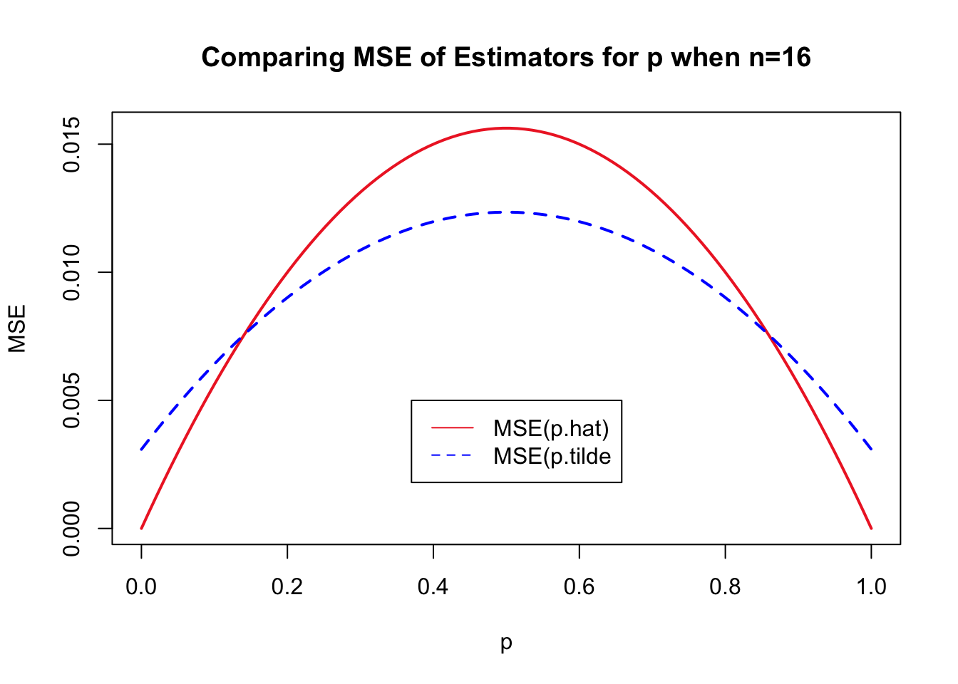

Figure 19.1: Comparing MSE of p-hat and p-tilde for X ~ Binom(16,p)

Question 8

Using the plots of \({\color{tomato}{\mbox{MSE}(\hat{p})}}\) and \({\color{dodgerblue}{\mbox{MSE}(\tilde{p})}}\) in Figure 19.1, identify the interval of \(p\) values where the MSE of \(\tilde{p}\) is less than the MSE of \(\hat{p}\).

Solution to Question 8

Question 9

Run run the code below for different values of \(n\) and say what happens to your choice of estimator as \(n\) gets larger.

#########################################
# adjust sample size n and run again
# what happens to mse as n gets larger?
#########################################
n <- ??  # sample size

####################################################
# you do not need to edit the rest of the code cell
####################################################

p <- seq(0, 1, length.out = 100)  # values of p

# formula for MSE of p-hat
mse.phat <- (p * (1 - p)) / n

# formula for MSE of p-tilde
mse.ptilde <- (n * p * (1 - p))/(n + 2)^2 + (1 - 2*p)^2/(n + 2)^2

# plot of MSE(p-hat)
plot(p, mse.phat,  
     type = "l",
     lwd =2,
     col = "firebrick2",
     main = "Comparing MSE of Estimators for p",
     ylab = "MSE")

# add plot of MSE(p-tilde)
lines(p, mse.ptilde,  
      lty=2, 
      lwd =2,
      col = "blue")

# add legend to plot
legend(0.37, 0.005, 
       legend=c("MSE(p.hat)","MSE(p.tilde"), 
       col=c("firebrick2","blue"), 
       lty=c(1,2), 
       ncol=1)

Solution to Question 9

Interpret the plots generated by the code above and answer the question.

Appendix: Proofs for Theorems

Theorem 15.1

If \(X_1\), \(X_2\), \(\ldots\) , \(X_n\) independently and identically distributed random variables, then

\[E\bigg[ \sum_{i=1}^n (X_i - \overline{X})^2 \bigg] = \sum_{i=1}^n E \big[ X_i^2 \big] - n E \big[ \overline{X}^2\big] .\]

Proof of Theorem 15.1

Let \(X_1\), \(X_2\), \(\ldots\) , \(X_n\) be independently and identically distributed random variables with \(\displaystyle \overline{X} = \frac{1}{n}\sum_{i=1}^n X_i\). The following properties are used in the proof that follows.

The linearity of the expected value of random variables gives

\[ E \bigg[ \sum_{i=1}^n (X_i) \bigg] = \sum_{i=1}^n \big( E \lbrack X_i \rbrack \big) = n\bar{X} \quad \mbox{and} \quad E \bigg[ \sum_{i=1}^n (X_i^2) \bigg] = \sum_{i=1}^n \big( E \lbrack X_i^2 \rbrack \big). \tag{20.1}\]

Recall properties of summation:

\[\sum_{i=1}^n (c a_i) = c \big( \sum_{i=1}^n a_i \big) \quad \mbox{and} \quad \sum_{i=1}^n c = nc. \tag{20.2}\]

We first expand the summation \(\sum_{i=1}^n (X_i - \overline{X})^2\) inside the expected value

\[\begin{aligned} E\bigg[ \sum_{i=1}^n (X_i - \overline{X})^2 \bigg] &= E \bigg[ (X_1 - \overline{X})^2 + (X_2 - \overline{X})^2 + \ldots + (X_n - \overline{X})^2 \bigg] \\ &= E \bigg[ (X_1^2 - 2X_1\overline{X} + \overline{X}^2) +(X_2^2 - 2X_2\overline{X} + \overline{X}^2) + \ldots + (X_n^2 - 2X_n\overline{X} + \overline{X}^2) \bigg] \end{aligned}\]

Regrouping terms, using the linearity of the expected value and properties of summation stated above, we have

\[E\bigg[ \sum_{i=1}^n (X_i - \overline{X})^2 \bigg] = \sum_{i=1}^n E(X_i^2) + E \bigg[ - 2 \overline{X}\left( {\color{tomato}{\sum_{i=1}^n X_i}} \right) + n \overline{X}^2 \bigg].\]

Since \(\overline{X} = \frac{1}{n} \sum_{i=1}^n X_i\), we have \({\color{tomato}{\sum_{i=1}^n X_i = n \overline{X}}}\), and therefore

\[\begin{aligned} E\bigg[ \sum_{i=1}^n (X_i - \overline{X})^2 \bigg] &= \sum_{i=1}^n E(X_i^2) + E \bigg[ - 2 \overline{X}\left( {\color{tomato}{n\overline{X}}} \right) + n \overline{X}^2 \bigg] \\ &= \sum_{i=1}^n E(X_i^2) + E \bigg[ -n \overline{X}^2\bigg]\\ &= \sum_{i=1}^n E(X_i^2) - n E \big[ \overline{X}^2\big] .\\ \end{aligned}\]

This concludes the proof!

Theorem 15.2

If \(X_1\), \(X_2\), \(\ldots\) , \(X_n\) are independently and identically distributed random variables with \(E(X_i) = \mu\) and \(\mbox{Var}(X_i) = \sigma^2\), then \(\displaystyle E \bigg[ \sum_{i=1}^n (X_i - \overline{X})^2 \bigg] = (n-1)\sigma^2\).

Proof of Theorem 15.2

We first apply Theorem 15.1 to begin simplifying the expected value of the sum of the squared deviations.

\[E\bigg[ \sum_{i=1}^n (X_i - \overline{X})^2 \bigg] = \sum_{i=1}^n {\color{dodgerblue}{ E \big[ X_i^2 \big]}} - n {\color{tomato}{E \big[ \overline{X}^2 \big]}}\]

From the variance property \(\mbox{Var}(Y) = E(Y^2) - \big( E(Y) \big)^2\), we know for any random variable \(Y\), we have \(E(Y^2) = \mbox{Var}(Y) + \big( E(Y) \big)^2\). Applying this property to each \(X_i\) and \(\overline{X}\) (which is a linear combination of random variables), we have

\[E\bigg[ \sum_{i=1}^n (X_i - \overline{X})^2 \bigg] = \sum_{i=1}^n \bigg( {\color{dodgerblue}{ \mbox{Var} \big[ X_i \big] + \left( E \big[ X_i \big] \right)^2 }} \bigg) - n \left( {\color{tomato}{\mbox{Var} \big[ \overline{X} \big] + \left( E \big[ \overline{X} \big]\right)^2}} \right)\]

From the first summation on the right side, we have \({\color{dodgerblue}{ \mbox{Var} \big[ X_i \big] + \left( E \big[ X_i \big] \right)^2 = \sigma^2 + \mu^2}}\). Recall from the Central Limit Theorem for Means, we have \(\mbox{Var} \big[ \overline{X} \big] = \frac{\sigma^2}{n}\) and \(E \big[ \overline{X} \big] = \mu\), and thus we have \({\color{tomato}{\mbox{Var} \big[ \overline{X} \big] + \left( E \big[ \overline{X} \big]\right)^2 =\frac{\sigma^2}{n} + \mu^2 }}\). Thus, we have

\[\begin{aligned} E\bigg[ \sum_{i=1}^n (X_i - \overline{X})^2 \bigg] &= \sum_{i=1}^n {\color{dodgerblue}{ \left( \sigma^2 + \mu^2 \right)}} - n \left( {\color{tomato}{\frac{\sigma^2}{n}}} + {\color{tomato}{ \mu^2}} \right) \\ &= n(\sigma^2 + \mu^2) - \sigma^2 - n\mu^2 \\ &= (n-1) \sigma^2. \end{aligned}\]

This concludes our proof!

Theorem 15.3

Let \(\hat{\theta}\) be an estimator for parameter \(\theta\). The mean squared error (MSE) is

\[\mbox{MSE} \big[ \hat{\theta} \big] = \mbox{Var} \big[\hat{\theta} \big] + \left( \mbox{Bias} \big[ \hat{\theta}\big] \right)^2.\]

Proof of Theorem 15.3

We begin with the definition, add and subtract \({\color{tomato}{E \big[ \hat{\theta} \big]}}\) inside the expected value, regroup terms inside the expected value, and finally break up the linear combination inside the expected value to get the result below.

\[\begin{aligned} \mbox{MSE} \big[ \hat{\theta} \big] &= E \big[ (\hat{\theta}-\theta)^2 \big] \\ &= E \bigg[ \left( \hat{\theta} {\color{tomato}{- E \big[ \hat{\theta} \big] + E \big[ \hat{\theta} \big]}} -\theta \right)^2 \bigg] \\ &= E \bigg[ \left( {\color{tomato}{(\hat{\theta} - E \big[ \hat{\theta} \big])}} + {\color{dodgerblue}{(E \big[ \hat{\theta} \big] -\theta)}} \right)^2 \bigg] \\ &= E \bigg[ {\color{tomato}{(\hat{\theta} - E \big[ \hat{\theta} \big])}}^2 + 2{\color{tomato}{(\hat{\theta} - E \big[ \hat{\theta} \big])}}{\color{dodgerblue}{(E \big[ \hat{\theta} \big] -\theta)}} + {\color{dodgerblue}{(E \big[ \hat{\theta} \big] -\theta)}}^2 \bigg] \\ &= E \bigg[ (\hat{\theta} - E \big[ \hat{\theta} \big])^2 \bigg] + 2 E \bigg[(\hat{\theta} - E \big[ \hat{\theta} \big]) (E \big[ \hat{\theta} \big] -\theta) \bigg] + E \bigg[ (E \big[ \hat{\theta} \big] -\theta)^2 \bigg] \end{aligned}\]

By definition of the variance, we have

\[{\color{tomato}{E \bigg[ (\hat{\theta} - E \big[ \hat{\theta} \big])^2 \bigg] = \mbox{Var} \big[ \hat{\theta} \big]}}. \tag{20.3}\]

By definition of bias of an estimator, we have

\[{\color{dodgerblue}{E \bigg[ (E \big[ \hat{\theta} \big] -\theta)^2 \bigg] = E \bigg[ \big( \mbox{Bias}(\hat{\theta}) \big)^2 \bigg] = \bigg( \mbox{Bias}(\hat{\theta}) \bigg)^2}}. \tag{20.4}\]

Note \(\mbox{Bias}(\hat{\theta})\) is a constant value which might be unknown, but it is not a random variable.
The expected value of a constant is the value of the constant, thus \(E \bigg[ \big( \mbox{Bias}(\hat{\theta}) \big)^2 \bigg] = \bigg( \mbox{Bias}(\hat{\theta}) \bigg)^2\).

\[{\color{mediumseagreen}{ \begin{aligned} E \bigg[ (\hat{\theta} - E \big[ \hat{\theta} \big]) (E \big[ \hat{\theta} \big] -\theta) \bigg] &= E \bigg[ \hat{\theta} \cdot E \big[ \hat{\theta} \big] - \hat{\theta} \cdot \theta - \bigg( E \big[ \hat{\theta} \big] \bigg)^2 + E \big[ \hat{\theta} \big] \cdot \theta \bigg] \\ &= E \big[ \hat{\theta} \big] E \big[ \hat{\theta} \big] - E \big[ \theta \big] E \big[ \hat{\theta} \big] - \bigg( E \big[ \hat{\theta} \big] \bigg)^2 + E \big[ \theta \big] E \big[ \hat{\theta} \big] \\ &= 0. \end{aligned} }} \tag{20.5}\]

Using the results in (Equation 20.3), (Equation 20.4), and (Equation 20.5), we have

\[\begin{aligned} \mbox{MSE} \big[ \hat{\theta} \big] &= {\color{tomato}{E \bigg[ (\hat{\theta} - E \big[ \hat{\theta} \big])^2 \bigg] }} + 2 {\color{mediumseagreen}{ E \bigg[(\hat{\theta} - E \big[ \hat{\theta} \big]) (E \big[ \hat{\theta} \big] -\theta) \bigg] }} + {\color{dodgerblue}{E \bigg[ (E \big[ \hat{\theta} \big] -\theta)^2 \bigg] }} \\ &= {\color{tomato}{\mbox{Var} \big[ \hat{\theta} \big]}} + 2 \cdot {\color{mediumseagreen}{0}} + {\color{dodgerblue}{\left( \mbox{Bias}(\hat{\theta}) \right)^2}} \\ &= \mbox{Var} \big[ \hat{\theta} \big] + \left( \mbox{Bias}(\hat{\theta}) \right)^2. \end{aligned}\]

This completes our proof!

Creative Commons License

Statistical Methods: Exploring the Uncertain by Adam Spiegler is licensed under a Creative Commons Attribution-NonCommercial-ShareAlike 4.0 International License.

Smith, J. W., Everhart, J. E., Dickson, W. C., Knowler, W. C. and Johannes, R. S. (1988) “Using the ADAP learning algorithm to forecast the onset of diabetes mellitus”. In Proceedings of the Symposium on Computer Applications in Medical Care (Washington, 1988), ed. R. A. Greenes, pp. 261–265. Los Alamitos, CA: IEEE Computer Society Press.↩︎