3.3: Sampling Distributions of Other Statistics

We have encountered situations where constructing sampling distributions for means and proportions are helpful. In addition to being useful summaries of data, both means and proportions are linear combinations of independent random variables.

• If \(X_1, X_2, \ldots , X_n\) are independent and identically distributed (i.i.d.) random variables (independently selected from the same population), then the sample mean is a linear combination of random variables,

\[\bar{X} = \frac{X_1 + X_2 + \ldots + X_n}{n}.\]

• If \(X \sim \mbox{Binom}(n, p)\), then the sample proportion is a multiple of one random variable,

\[\widehat{P} = \frac{X}{n}.\]

Thus for proportions and means, we can derive the Central Limit Theorem (CLT) to describe the mean and standard error (spread) of sampling distributions by applying properties of expected value and variance of independent random variables:

\[E(aX + bY) = aE(X) + bE(Y) \qquad \mbox{and} \qquad \mbox{Var}(aX + bY) = a^2\mbox{Var}(X) + b^2 \mbox{Var}(Y).\]

There many other statistics that may be more relevant to study to other situations. Generalizing sampling distributions to other statistics will allow us to explore a bigger variety of questions. Even if we cannot derive formulas that describe the mean and variance of other sampling distributions, we can construct a sampling distribution using a simulation. Sometimes simulations bring to light patterns and conjectures that we can try to verify and prove analytically.

Simulation for Sampling Distributions

---

We can apply the same method as we used with constructing sampling distributions for means and proportions to create a sampling distribution for any statistic. The general process is as follows:

1. Pick a random sample size \(n\) from population \(X\).
2. Calculate some statistic(s) of interest from the sample.
3. Repeat. Generate many random samples (each size \(n\)) and calculate the statistic(s) of interest from each sample.

We previsouly considered the sampling distribution for the mean wait time between trains. In that example, the wait time between trains was exponentially distributed with a mean of \(4\) minutes between trains. Thus, the rate parameter is \(\lambda = \frac{1}{4}\). We sample from the population of \(Y \sim \mbox{Exp} \left( \frac{1}{4} \right)\) which is skewed to the right.

Run the code cell below to create a sampling distribution for the mean time between trains with samples size \(n=50\).

• We will generate 10,000 random samples, and the mean of each will be stored in the vector samp.mean.
• The for loop includes the steps for creating a sampling distribution:
  • Pick a random sample stored in time.sample using rexp(50, 1/4).
  • Calculate the mean of the sample with mean(time.sample).
• No output is printed to screen after running the code cell below since the values are being stored in samp.mean.

# creates an empty vector to store results
samp.mean <- numeric(10000)

# a for loop that generates 10000 random samples 
# each size n=50, and calculates the sample mean.
for (i in 1:10000)
{
  time.sample <- rexp(50, 1/4)  # Step 1: Randomly picks 50 values from Exp(1/4)
  samp.mean[i] <- mean(time.sample)  # Step 2: calculate sample mean
}

Graphical Summary of Results of Simulation

---

Run the code cell below to generate side-by-side plots of the pdf of the population \(Y \sim \mbox{Exp}(1/4)\) and a sampling distribution for the mean with \(n=50\).

par(mfrow=c(1,2))  # arrange plots side by side

# plot population
y <- seq(0, 6, 0.01) 
plot(y, dexp(y), type = "l",
     xlab = "Y, wait time (in min)",
     main = "Population, Y ~ Exp(1/4)")

# plot the sampling distribution of means
hist(samp.mean, 
     breaks = 20,
     xlab = "Mean Wait Time (n=50)",
     main = "Dist. of Sample Means")
abline(v = mean(samp.mean), col = "blue", lwd = 2)  # center of sampling dist of mean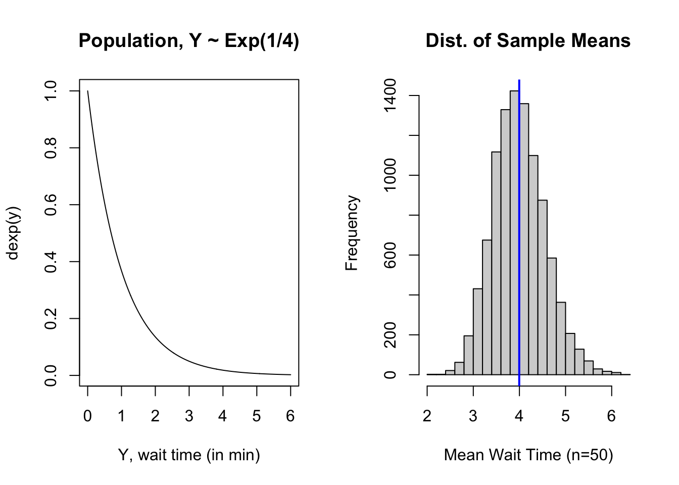

Simulation for Sampling Distribution for Median

---

Since wait times between trains are skewed to the right, the sample means will be more heavily influenced by outliers that are biased to the right. The median is the 50th percentile of the data, and it is not as sensitive to outliers. We might want to consider a sampling distribution for the median if we want to consider a measure of center that is less influenced by outliers.

Question 1

---

Complete the partially completed code cell below to generate a sampling distribution for the median weight time between trains using samples size \(n=50\). You should continue to assume the time between successive trains is exponentially distributed with a mean time of 4 minutes between successive trains.

Solution to Question 1

---

Replace each of the three ?? in the code cell below with appropriate code. Then run the completed code to create and plot a sampling distribution for the sample median for samples size \(n=50\).

# creates an empty vector to store results
samp.median <- numeric(10000)

# a for loop that generates 10000 random samples 
# each size n=50, and calculates the sample median
for (i in 1:10000)
{
##################################
# Replace both ?? in the for loop
##################################
  time.sample <- ??  # Step 1: Pick random sample from population
  samp.median[i] <- ??  # Step 2: Calculate sample statistic
}


# plot the sampling distribution
#####################################
# Replace the ?? in the hist command
#####################################
hist(??, 
     breaks = 20,
     xlab = "Median Wait Time (n=50)",
     main = "Dist. of Sample Means")
abline(v = mean(samp.median), col = "red", lwd = 2, lty = 2)  # center of sampling dist of median
abline(v = mean(samp.mean), col = "blue", lwd = 2, lty = 2)  # center of sampling dist of mean

Question 2

---

Based on the plot of the sampling distribution for the median plotted above, comment on the significance of the red and blue vertical lines included in the plot.

• What quantity is the red line representing? What quantity is the blue line representing?
• Compare the locations of the two lines. Why is the blue line to the right of the red line? Explain why this makes sense in this context.

Solution to Question 2

---

Question 3

---

Based on the results of the sampling distribution for the median stored in samp.median in Question 2 answer the following questions.

Question 3a

---

Create a qq-plot of the sampling distribution and comment on whether shape of the sampling distribution for median is normal or not.

Solution to Question 3a

---

# create a qq-plot of the sampling dist for median
# interpret the output after writing/running code

Question 3b

---

Compute the standard error of the sampling distribution for medians and the standard error for the sampling distribution for means. Compare both values. Which is bigger and why does that make practical sense?

Tip

Results for the sampling distribution of the mean wait time between trains were stored in samp.mean in an earlier code cell. Be sure you have run that code and stored those results.

Solution to Question 3b

---

# calculate both standard errors
# interpret the output after writing/running code

Simulation for Sampling Distribution for Variance

---

Variance is one of the most frequently used measurements for the spread of a distribution. If we pick a random sample of values \(X_1, X_2, \ldots , X_n\) from a population, it is natural to consider how much variation can we expect in the spread of values (measured by variance) for different random samples of size \(n\). The variance is not a linear combination of random variables \(X_1, X_2, \ldots , X_n\), so we cannot use the same properties of expected value and variance that we applied to derive the Central Limit Theorem for means and proportions. Instead, we will use a simulation based method to investigate properties of a sampling distribution for sample variances.

Question 4

---

Cholesterol is a fat-like substance present in all cells in your body. A blood test is used to measure cholesterol levels. The distribution of cholesterol levels for adults age 20 or older is approximately normally distributed with a mean of 200 mg/dL and standard deviation 40 mg/dL. Let \(X\) be the cholesterol level of a randomly selected adult age 20 or above. Thus, we have \(X \sim N(200, 40)\).

Question 4a

---

Complete the partially completed code cell below to generate a sampling distribution for the sample variance of cholesterol level using samples size \(n=25\).

Solution to Question 4a

---

Replace each of the three ?? in the code cell below with appropriate code. Then run the completed code to create and plot a sampling distribution for the sample variance for samples size \(n=25\).

# creates an empty vector to store results
samp.var <- numeric(10000)

# a for loop that generates 10000 random samples 
# and calculates the sample variance
for (i in 1:10000)
{
##################################
# Replace both ?? in the for loop
##################################
  cholest.sample <- ??  # Step 1: Pick random sample from population
  samp.var[i] <- ??  # Step 2: Calculate sample statistic
}


# plot the sampling distribution
#####################################
# Replace the ?? in the hist command
#####################################
hist(??, 
     breaks = 20,
     xlab = "Variance of Cholesterol (n=25)",
     main = "Dist. of Sample Variance")
abline(v = mean(samp.var), col = "red", lwd = 2, lty = 2)  # center of sampling dist of variance

Question 4b

---

Based on the results of the sampling distribution for the sample variance stored in samp.var after running the code above:

• Calculate the mean and standard error of the sampling distribution for the sample variance when \(n=25\).
• Create a qq-plot and comment on whether or not the sampling distribution for the sample variance appears to be normal or not.

Solution to Question 4b

---

# calculate mean and standard error of 
# sampling distribution of sample variance

# create a qq-plot of the sampling dist for sample variance
# interpret the output after writing/running code

Deriviving Formulas for Sampling Distributions

---

In the previous examples involving sample median and variance, we are able to analyze properties of the sampling distribution of those statistics by simulating the creation of a sampling distribution. We can always use simulations to approximate sampling distributions, even if we do not have a formal theorem or formulas that describe the distribution for those sample statistics. With some statistics, such as sample means and sample proportions, we can use properties of random variables to derive theory and formulas that describe properties of the sampling distribution. In situations where we can theoretically model sampling distributions, technology is not required to describe the sampling distribution. We explore some additional statistics, namely the maximum of a sample, and derive formulas we can use to describe a sampling distribution of maximum values.

Sampling Distribution for the Maximum

---

Frequently we are interested in the sample maximum value, denoted \(\color{dodgerblue}{X_{\rm{max}}}\), of a random sample. For example, if we pick a random sample of five values, \(\left\{ 11, 18, 2, 31, 25 \right\}\), then we have the statistics \(X_{\rm{min}} = 2\) and \(X_{\rm{max}} = 31\). A sampling distribution for the sample maximum would be the distribution of maximum values obtained from samples when we independently pick many random samples, each size \(n\), from the same population.

Question 5

---

Let \(F\) denote the cumulative distribution function (cdf) for a continuous random variable \(X\). Derive the cdf for \(X_{\rm{max}}\), the maximum of a random sample \(X_1,X_2, \ldots, X_n\), with each \(X_i\) independently picked from the same population \(X\) that has cdf \(F(x)\).

An outline of a proof is provided below. In the solution space below, fill in missing explanations for each step of the proof.

\[\begin{aligned} F_{X_{\rm{max}}} (a) &= P(X_1 \leq a, X_2 \leq a, \ldots, X_n \leq a) & \mbox{Explanation 1} \\ &= P\big( (X_1 \leq a) \cap (X_2 \leq a) \cap \ldots \cap (X_n \leq a) \big) & \mbox{Explanation 2}\\ &= P(X_1 \leq a) \cdot P(X_2 \leq a) \cdot \ldots \cdot P(X_n \leq a) & \mbox{Explanation 3}\\ &= F(a) \cdot F(a) \cdot \ldots \cdot F(a) & \mbox{Explanation 4}\\ &= \big( F(a) \big)^n \end{aligned}\]

Solution to Question 5

---

Explanation 1:

Explanation 2:

Explanation 3:

Explanation 4:

Question 6

---

Using the result from the previous problem, find \(\displaystyle f_{X_{\rm{max}}} (a)\), the probability density function (pdf) for the maximum of a random sample. Your answer will depend on both \(F\) and \(f\), the corresponding cdf and pdf, respectively, of \(X\).

Hint: Recall the general relation between cdf’s and pdf’s of continuous random variables.

Solution to Question 6

---

Summarizing Results for \(X_{\rm{max}}\)

---

Let \(F\) denote the cumulative distribution function (cdf) for a continuous random variable \(X\), and let \(X_{\rm{max}}\) denote the maximum of a random sample \(X_1,X_2, \ldots, X_n\), where each \(X_i\) is independently picked from population \(X\). Then the sample maximum, \(X_{\rm{max}}\), will have:

• Cumulative distribution function \(\displaystyle F_{X_{\rm{max}}} (a) = \big( F(a) \big)^n\).
• Probability density function \(\displaystyle f_{X_{\rm{max}}} (a) = n \left( F(a) \right)^{n-1} f(a)\).

Question 7

---

Let \(X\) be a random variable with continuous uniform distribution \(\mbox{Unif}(0,1)\). Answer the questions below regarding the distribution \(X\) and the distribution of sample maximum, \(X_{\rm{max}}\), for \(n=10\).

Question 7a

---

What are the cdf and pdf, \(F(x)\) and \(f(x)\) respectively, of \(X \sim \mbox{Unif}(0,1)\)? Hint: See useful properties of continuous uniform distributions.

Solution to Question 7a

---

Question 7b

---

If we pick a random sample of size \(n=10\), how likely is it that \(X_{\rm{max}}\) is greater than or equal to \(0.9\)?

Tip

Use the formulas from your answer to Question 7a and make use of the formulas for the cdf and/or pdf we derived for \(X_{\rm{max}}\).

Solution to Question 7b

---

Sample Maximum: Comparing Theory with Simulation

---

In Question 8 below, we check our analytic solutions for Question 7 using a statistical simulation.

Question 8

---

Replace each of the three ?? in the code cell below with appropriate code. Then run the completed code to create and plot a sampling distribution for the sample maximum for samples size \(n=10\) from \(X \sim \mbox{Unif}(0,1)\).

Solution to Question 8

---

Replace each of the three ?? in the code cell below and run to create and plot a sampling distribution for the sample maximum for samples size \(n=10\) picked from \(X \sim \mbox{Unif}(0,1)\).

# creates an empty vector to store results
samp.max <- numeric(10000)

# a for loop that generates 10000 random samples 
# calculates the sample maximum
for (i in 1:10000)
{
##################################
# Replace both ?? in the for loop
##################################
  temp.sample <- ??  # Step 1: Pick random sample from population
  samp.max[i] <- ??  # Step 2: Calculate sample statistic
}


# plot the sampling distribution
#####################################
# Replace the ?? in the hist command
#####################################
hist(??, 
     breaks = 20,
     xlab = "Maximum of Sample (n=10)",
     main = "Dist. of Sample Max")
abline(v = 0.9, col = "red", lwd = 2, lty = 2)  # marking x_max = 0.9

Question 9

---

Based on the results of the sampling distribution for the sample maximum stored in samp.max after running the code above:

• Use your sampling distribution from Question 8 to approximate \(P(X_{\rm{max}} \geq 0.9)\).
  • Hint: Use a logical test involving samp.max and either a sum() or mean() command.
• Compare your approximation to the exact value you found in Question 7b.

Solution to Question 9

---

# use results in samp.max to
# approx P(X_max >= 0.9)

Sampling Distribution for Goodness-of-Fit

---

The stop-and-frisk policy is the practice of temporarily stopping, questioning, and possibly searching civilians suspected of carrying illegal possessions such as drugs and weapons. The program has come under scrutiny in many cities regarding claims of racial-profiling. We investigate the following question:

Does the stop-and-frisk program in New York City seem to profile people based on race?

In 2022, 15,102 stops were recorded by NYPD, and these stops are broken down by race in the table below.

Race	2022 NYPD Stops1	NYC Population2
Black	8,863	\(0.23\)
Latinx	4,477	\(0.29\)
White	1,077	\(0.32\)
Asian/Pacific Islander	320	\(0.14\)
Mixed/Other	365	\(0.02\)
Total	15102	1

• In the code cell below, we save the data in the table to two vectors observe and prop.
• Be sure to run the code cell below in order to answer the questions that follow.

observe <- c(8863, 4477, 1077, 320, 365)  # vector of observed values
prop <- c(0.23, 0.29, 0.32, 0.14, 0.02)  # vector of population proportions

In the jury example from our exploration with sampling distributions for a single proportion, we considered whether people that identify their political party as Independent have fair representation. Political party was a binary variable (Independent or Not). Perhaps a more useful question to explore is whether the jury has a good representation of all political affiliations, not just Independents. When working with a categorical variable that has more than two categories, such as race or political affiliation, we need to consider more than a single proportion. Rather than consider a single proportion, we can conduct a chi-square goodness-of-fit test to measure how well the random sample resembles the population as far as what proportion of observations are in each category. We assume the categories are mutually exclusive (an observation cannot belong to multiple categories), and thus the sum of all proportions is 1.

Question 10

---

This question guides us through the calculation of a statistic to measure how well racial demographics of the people stopped by NYPD in 2022 match the overall racial demographics of NYC in 2022.

Question 10a

---

First, we calculate the expected totals for each racial category. Each expected total is the proportion of the population in the group, \(p_i\), times the total sample size, \(n\).

• Complete the code cell below to calculate and store each expected value \(\mbox{Expected}_i = n p_i\) in the vector expect.
• After running the code, make sure the output matches the values in expected column in the table below.

Race	Observed	NYC Population	Expected
Black	8,863	\(0.23\)	\(3473.46\)
Latinx	4,477	\(0.29\)	\(4379.58\)
White	1,077	\(0.32\)	\(4832.64\)
Asian/Pacific Islander	320	\(0.14\)	\(2114.28\)
Mixed/Other	365	\(0.02\)	\(302.04\)
Total	15102	1	\(15102\)

Solution to Question 10a

---

n <- sum(observe)  # sample size = total number of observed
expect <- ??  # compute vector of expected totals
expect    # print values to screen

Question 10b

---

Next, we calculate the difference in the observed and expected totals for each category. Since we do not want positive and negative differences to cancel out, we square each distance, \((O_i - E_i)^2\).

• Complete the code cell below to calculate and store the each of the squared differences \((O_i - E_i)^2\) in the vector named sq.diff.
• Run the completed code cell before continuing to the next part.

Solution to Question 10b

---

sq.diff <- ??  # compute vector of (O-E)^2 values
sq.diff  # print values to screen

Question 10c

---

Since larger categories are going to have larger differences, we consider each squared distance \((O_i - E_i)^2\) relative to the expected size of the category, \(E_i\).

• Complete the code cell below to calculate and store each ratio of squared difference over expected count, \(\frac{(O_i - E_i)^2}{E_i}\), in the vector named relative.diff.
• After running the code, you can check your output with the values in the \((E-O)^2/E\) column in the table below Question 10d.

Solution to Question 10c

---

relative.diff <- ??  # compute vector of (O-E)^2/E values
relative.diff  # print values to screen

Question 10d

---

Finally, sum all the ratios in relative.diff together to compute a single statistic called the chi-square test statistic that is denoted \(\color{dodgerblue}{\chi^2}\),

\[\color{dodgerblue}{\chi^2 = \sum_{i} \frac{(O_i - E_i)^2}{E_i}}.\]

• Complete the code cell below to sum together all \(\frac{(O_i - E_i)^2}{E_i}\) previously computed and stored in the vector relative.diff.
• After running the code, you can check your output with the total of the \((E-O)^2/E\) column in the table below.

Solution to Question 10d

---

nyc.chi.sq <- ?? # sum together all (O-E)^2/E to compute chi-sq stat
nyc.chi.sq   # print value to screen

Race	Observed	NYC Population	Expected	\((E-O)^2/E\)
Black	8,863	\(0.23\)	\(3473.46\)	\(8362.6\)
Latinx	4,477	\(0.29\)	\(4379.58\)	\(2.167\)
White	1,077	\(0.32\)	\(4832.64\)	\(2918.7\)
Asian/Pacific Islander	320	\(0.14\)	\(2114.28\)	\(1522.7\)
Mixed/Other	365	\(0.02\)	\(302.04\)	\(13.124\)
Total	15102	1	\(15102\)	\(\color{dodgerblue}{12819.26}\)

Simulating a Distribution of Sample \(\chi^2\)

---

1. Pick a random sample size \(n\) from the population (NYC in 2022).

temp <- sample(c("Black", "Latinx", "White", "Asian/Pacific Islander", "Mixed/Other"),
                      size = 15102,  
                      replace = TRUE, 
                      prob = c(0.23, 0.29, 0.32, 0.14, 0.02))

2. Calculate the chi-square test statistic of the sample as described in the previous section.

o1 <- sum(temp == "Black")
o2 <- sum(temp == "Latinx")
o3 <- sum(temp == "White")
o4 <- sum(temp == "Asian/Pacific Islander")
o5 <- sum(temp == "Mixed/Other")

temp.obs <- c(o1, o2, o3, o4, o5)
rel.diff <- (temp.obs - expect)^2 / expect
sample.chi <-sum(rel.diff)

3. Repeat many (1,000) times.

dist.chi <- numeric(1000) # creates an empty vector to store results
n <- 15102  # total number of observed
prop <- c(0.23, 0.29, 0.32, 0.14, 0.02)  # nyc racial demographics
expect <- n * prop  # sample size * population prop

# a for loop that generates 1000 random samples 
for (i in 1:1000)
{
  temp<- sample(c("Black", "Latinx", "White", "Asian/Pacific Islander", "Mixed/Other"),
                      size = n,  
                      replace = TRUE, 
                      prob = c(0.23, 0.29, 0.32, 0.14, 0.02))
  o1 <- sum(temp == "Black")
  o2 <- sum(temp == "Latinx")
  o3 <- sum(temp == "White")
  o4 <- sum(temp == "Asian/Pacific Islander")
  o5 <- sum(temp == "Mixed/Other")
  temp.obs <- c(o1, o2, o3, o4, o5)
  rel.diff <- (temp.obs - expect)^2 / expect
  dist.chi[i] <-sum(rel.diff)
}

hist(dist.chi,  # plot stored sample statistics
     breaks = 20,  # use 20 breaks
     xlab = "Sample Goodness-of-Fit",  # x-axis label
     main = "Sampling Distribution of Chi-Squared Statistics",  # main label
     freq = FALSE)  # plot relative frequencies (density) on y-axis

abline(v = 12819.26, col = "red", lwd = 2, lty = 2)  # draws vertical line at observed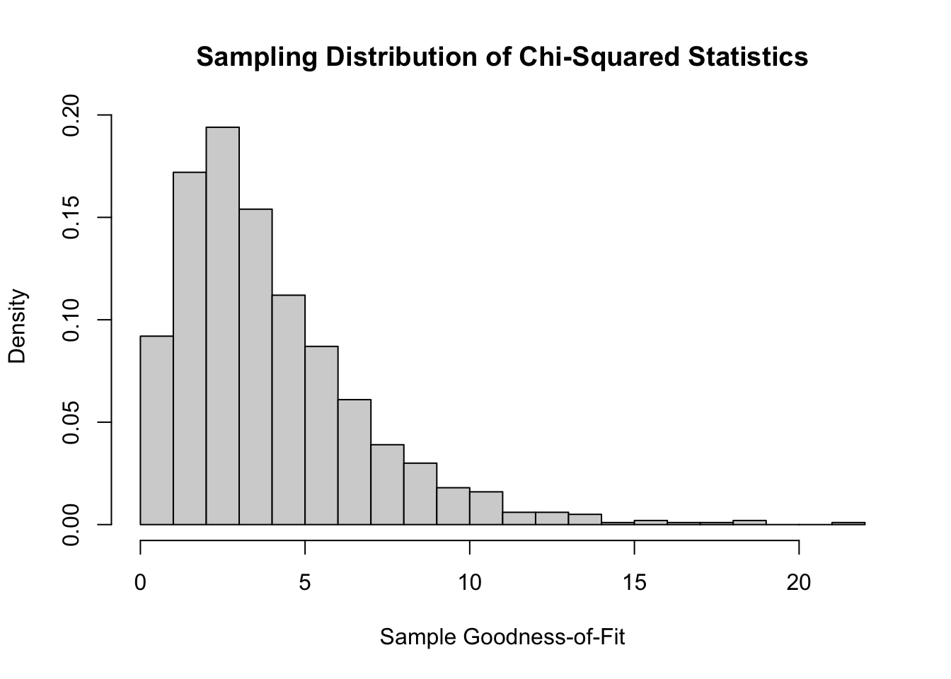

Interpreting Results

---

Based on the stop-and-frisk data from NYPD in 2022, the chi-square test statistic was \(12,819.26\). That is off the chart compared to the chi-square statistics we obtained from all the other random samples of the same size. The figure below shows just how extreme the chi-square test statistic and far removed it appears from samples that are randomly picked from the same population. This does not necessarily imply there is racial discrimination as that is a very complex question. There are other factors we need to consider, and this is an important question that requires more analysis and looking deeper into the data.

hist(dist.chi,  # plot stored sample statistics
     breaks = 20,  # use 20 breaks
     xlab = "Sample Goodness-of-Fit",  # x-axis label
     main = "Sampling Distribution of Chi-Squared Statistics",  # main label
     freq = FALSE,  # plot relative frequencies (density) on y-axis
     xlim = c(0, 14500),
     xaxt = 'n')
axis(1, at=seq(0, 13000, 1000), pos=0)  # customize ticks on x-axis
abline(v = 12819.26, col = "red", lwd = 2, lty = 2)  # draws vertical line at observed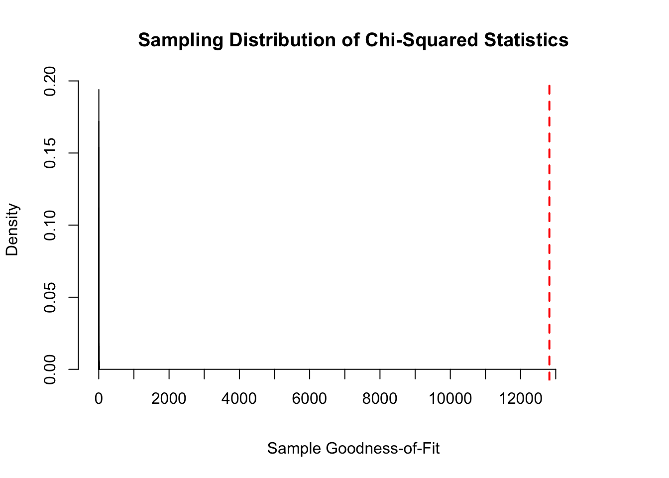

---

Statistical Methods: Exploring the Uncertain by Adam Spiegler is licensed under a Creative Commons Attribution-NonCommercial-ShareAlike 4.0 International License.

---

1. Data from (NYPD Stop, Ask, and Frisk Data 2022

2. Data from US Census Data