6.4: Parametric Tests for Two Populations

When we discussed parametric methods for modeling null distributions that we used to calculate p-values, we focused on tests involving a single population, such as claims about a single mean or a single proportion. Often in statistics we would like to investigate whether one variable is associated to another. For example:

Q1: Is a new medication more effective at preventing disease than current treatments?
Q2: Is there a gender pay gap in the US?
Q3: Is there a region in the North Atlantic where storm strength is greatest?

If we are using one variable to help us understand or predict the values (or category) of another variable:

We call the first variable the explanatory, independent, or predictor variable.
The second the response or dependent variable.
Different categories of a predictor variable are called treatments or levels.

In this section, we develop a parametric method to perform hypothesis tests that compare the response of one variable for two different levels of an explanatory variable.

The explanatory variable is categorical, and we compare two levels to each other.
The response variable may be a categorical or a quantitative variable.
- For a quantitative response, we make claims about a difference in means.
- For a categorical response, we make claims about a difference in proportions.

Questions that Compare Two Populations

In many cases, the explanatory variable of interest in our question has more than just two levels. We can apply hypothesis tests on two populations to compare two levels of the explanatory variable. Often the researchers have a goal in mind, and they choose which two levels they would like to compare and/or how the levels are defined. Another group of researchers might approach the same statistical question from a different perspective and choose a different set up.

Question 1

Suppose the explanatory variable for statistical questions Q1, Q2, and Q3 are:

Q1: Medication Type
Q2: Gender
Q3: Latitude

In the questions below, set up null and alternative hypothesis (in words and symbolically) to perform a hypothesis test to answer the statistical question.

Question 1a

Q1: Is a new medication more effective at preventing disease than current treatments?

In general, we might be interested in comparing several treatments. For example, the variable Medication Type could have four different levels: Treatment A, Treatment B, Treatment C, and No Treatment. Within our hypothesis test framework, we can compare two different treatments types. Set up hypotheses for the following question:

Does xylitol (a sweetener) reduce ear infections in children compared to no treatment (control)?

Solution to Question 1a

$H_0$:
$H_a$:

Question 1b

Q2: Is there a gender pay gap in the US?

The explanatory variable Gender may be gathered using different methods: free response question, multiple choice question (with various ways of defining the choices), or pulled directly from available records. Suppose we would like to focus on identifying if there is a pay gap between men and women that have just completed a bachelor’s degree in the US. Set up hypothesis for the following question:

Do women that have recently completed a bachelor’s degree in the US get paid less, on average, compared to men that have recently completed a bachelor’s degree?

Note

The median is often used as the measure of center to summarize income since the distribution of income is typically heavily skewed. Outliers will have a bigger influence in the analysis if we compare means. With the median, outliers have as much influence as any other observation. However, there is no parametric method for testing claims about medians.

Solution to Question 1b

$H_0$:
$H_a$:

Question 1c

Q3: Is there a region in the North Atlantic where storm strength is greatest?

The explanatory variable Latitude is typically a quantitative variable given in degrees north or south of the equator. There are many different ways a researcher can define different regions, and how they define those regions depends on the data available and their research goals. Set up hypothesis for the following question:

Is the storm pressure different, on average, for storms in the North Atlantic above the Tropic of Cancer compared to those below the Tropic of Cancer?

Solution to Question 1c

$H_0$:
$H_a$:

Hypothesis Tests for Comparing Two Populations

When doing a hypothesis test for a difference between population means or two population proportions, we apply the same steps as with previous tests. See Appendix A for a summary of the steps below.

Set up hypotheses.
- $H_0$: There is no difference between the two levels.
- $H_a$: There is a difference between the two levels.
Collect data, calculate the difference in sample statistics, and find a test statistic.
Calculate the p-value.
Based on the significance level, $\alpha$, make a conclusion.
Summarize the results in context.

In our previous work with hypothesis tests on two populations, we used two-sample permutations tests to find standardized test statistics and p-values in steps 2 and 3. We now devise parametric methods for hypothesis tests that compare two populations.

A General Test Statistic

We can apply the Central Limit Theorem, CLT, to standardize the test statistic and calculate p-values using the same strategy as the parametric approach for testing claims about a single population. We begin by assuming the claim in the null hypothesis is true:

$H_0$: There is no difference. For example, $\mu_1 - \mu_2 =0$ or $p_1 -p_2 = 0$.

The standardized test statistic is the $z$-score or t-test statistic corresponding to the observed difference in sample statistics:

\[{\color{dodgerblue}{\mbox{stand test stat} = \frac{ (\mbox{diff in sample stats}) - ({\color{tomato}{\mbox{diff in null claim}}})}{\mbox{SE of Null Dist}} = \frac{ (\mbox{diff in sample stats}) - {\color{tomato}{0}}}{\mbox{SE of Null Dist}}}}.\]

To calculate the standardized test statistic, we consider the following questions:

Do the samples satisfies conditions for CLT?
What is the correct probability distribution to use, a t-distribution or a normal distribution?
What is the difference in observed sample statistics?
What is an estimate for the standard error of the null distribution?

Difference in Two Means: Parametric Method

Question 2

If we are doing a test on a difference of means from two independent populations, then the null claim is $H_0$: $\mu_1 - \mu_2=0$ and recall the CLT for a difference in means is

\[\overline{X}_1 - \overline{X}_2 \sim N \left( {\color{tomato}{\mu_1 - \mu_2}} , {\color{dodgerblue}{\mbox{SE}}} \right) = N \left( {\color{tomato}{0}} , {\color{dodgerblue}{\sqrt{\frac{\sigma_1^2}{n_1} + \frac{\sigma_2^2}{n_2}}} } \right).\] Suppose we are performing a test on the difference of two independent means, $\mu_1 - \mu_2$, and the population variances $\sigma_1^2$ and $\sigma_2^2$ are unknown.

What are reasonable estimates to use in place of $\sigma_1^2$ and $\sigma_2^2$?
What is a formula for estimating the standard error of the null distribution?
Should we use a t-distribution or normal distribution to approximate the null distribution?

Based on your answers to the previous questions, fill in the blanks label (i), (ii), (iii), and (iv) to give a formula for standardized test statistic. In blank (i), enter either $z$ or $t$ depending on whether a normal or t-distribution is appropriate.

\[{\color{dodgerblue}{\mbox{(i)} = \frac{ (\mbox{diff in sample stats}) - ({\color{tomato}{\mbox{diff in null claim}}})}{\mbox{SE of Null Dist}} = \frac{ \mbox{(ii)} - {\color{tomato}{\mbox{(iii)}}}}{\mbox{(iv)}}}}.\]

Solution to Question 2

Complete the formula for the standardized test statistic:

Choose either $z$ or $t$ for blank (i).
Blank (ii) is ??
Blank (iii) is ??
Blank (iv) is ??

Question 3

We return to our statistical question and hypothesis from Question 1b regarding a possible gender pay gap in the US. We collect data from a random sample of people that completed their bachelor’s degree in 2021 and compare the starting salaries of men and women in the sample. A sample of 154 women have a mean income of $\$52,\!266$ with standard deviation $\$15,\!510$ A sample of 122 men have a mean income of $\$64,\!022$ with a standard deviation of $\$16,\!890$.

Is there enough evidence to support the claim that women who have recently completed a bachelor’s degree in the US get paid less, on average, compared to men who have recently completed a bachelor’s degree? Test using a significance level of $\alpha=0.05$.

Note

The statistical question in this example as well as the data are motivated by an analysis of students that earned a bachelor’s degree in the US in 2021 by the National Association of Colleges and Employers (NACE).

Solution to Question 3

Using the hypotheses you set up in Question 1b, answer the following:

Based on the sample data, compute the standardized test statistic.

# calculate standardized test statistic

Based on your standardized test statistic, compute the p-value.

# compute p-value

Make a decision and summarize the results in the context of this example.

Using `t.test()` to Compare Two Populations

To calculate a p-value for a test on the difference of means from two independent populations with unknown variances, we can calculate the t-test statistic

\[{\boxed{\color{dodgerblue}{{\color{tomato}{t}} = \frac{ \mbox{diff in sample stats} - 0}{\mbox{SE of Null Dist}} = \dfrac{(\bar{x}_1 - \bar{x}_2) - 0 }{\sqrt{\frac{{\color{tomato}{s_1}}^2}{n_1} + \frac{{\color{tomato}{s_2}}^2}{n_2}}}}}}.\]

In Question 3, you were conveniently provided numerical summaries of each sample that we substituted into the formula for the t-test statistic. Then we can err on the side caution and choose the degrees of freedom, $df$, to be the smaller of either $\mathbf{n_1-1}$ or $\mathbf{n_2-1}$.

If we have access to all the sample data (not just summaries), then we can load the sample data into R and use the t.test() function to calculates both the t-test statistic and p-value using a more accurate approximation for $df$ obtained using Welch’s approximation.

Samples Stored as Separate Vectors

In R, we can use the command t.test(x1, x2, alt = [direction]).

Samples are stored in independent vectors x1 and x2.
Set the option alt based on the inequality used in $H_a$.
- Use "greater" for right-tail test.
- Use "less" for left-tail test.
- Use "two.sided" for a two-tail test.
- If you do not indicate any alt option, the default is a two-tailed test.
The default is mu=0 which is exactly what we want, so we do not specify this option.

Subsetting Samples Inside `t.test()`

Frequently, we would like to compare the means of a quantitative response variable, denoted quant, for two different levels of a categorical explanatory variable, denoted categorical, in the data frame named data.name. The t.test() function can simultaneously subset the quant data into two independent samples (one for each level of category) and then perform a hypothesis test for the difference in two means:

t.test(quant ~ categorical, data = data.name, alt = [direction])

Caution

If the categorical variable has exactly two levels, then the command t.test(quant ~ categorical, data = data.name, alt = [direction]) works as desired. However, if categorical has more than two levels, this results in an error. If there are more than two levels, you can first subset or filter the data and then use t.test().

Question 4

We use the storms data set from the NOAA Hurricane Best Track Data in the dplyr package to test if the storm pressure is different, on average, for storms in the North Atlantic above the Tropic of Cancer compared to those below the Tropic of Cancer.

Run the code cell below to load the dplyr package (which should already be installed).

library(dplyr)  # load dplyr package

Question 4a

Run the code cell below to calculate the p-value of the sample data in storms. Interpret the meaning of the output.

t.test(pressure ~ lat, data = storms, alt = "two.tail")

Solution to Question 4a

Question 4b

The Tropic of Cancer is the most northerly circle of latitude on Earth at which the Sun can be directly overhead. The position of this circle is constantly wobbling just slightly. The Tropic of Cancer is currently located at $23.43623^{\circ}$ north of the Equator.

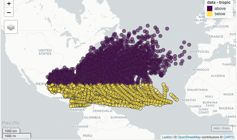
Creating Levels for the Explanatory Variable with `mutate()`

The code cell use the mutate() function that is in the dplyr package to create and add a new categorical variable, we name tropic, consisting of two levels (above and below) depending on whether the storm’s location is above or below the Tropic of Cancer. Then the tapply() function is used to calculate separate means for the sample of storms above and below the Tropic of Cancer.

Note

The data frame storms and mutate() script are both in the dplyr package. Be sure you have already run library(dplyr) before running the code cell below.

# create and add new variable tropic to storms
storms <- mutate(storms, 
                 tropic = case_when(lat < 23.43623 ~ 'below',  # below is assigned if lat < 23.43623
                                    lat > 23.43623 ~ 'above'))  # above is assigned if lat > 23.43623

storms$tropic <- factor(storms$tropic)  # ensure tropic stored as categorical factor
tapply(storms$pressure, storms$tropic, mean)  # compare mean pressures

After running the code cell above, complete the code cell below to create side-by-side box plots of the distributions of storm pressures above and below the Tropic of Cancer.

Solution to Question 4b

Replace each ?? with an appropriate variable or data frame name.

boxplot(?? ~ ??, data = ??)

Question 4c

Fill in the t.test() function below to compute the test statistic and corresponding p-value based on the sample data in storms to test the hypothesis in Question 1c

Solution to Question 4c

Complete and run the code cell below.

t.test(?? ~ ??, data = ??, alt = ??)

Question 4d

Based on the output in Question 4c, summarize the result of this test in practical terms. Use a significance level of 5%.

Solution to Question 4d

Difference in Proportions: A Parametric Method

If we are doing a test on a difference of two proportions, then the null claim is $H_0$: $p_1 - p_2=0$. We use the difference in sample proportions, ${\color{dodgerblue}{\hat{p}_1 - \hat{p}_2}}$, as the test statistic:

\[{\color{dodgerblue}{\mbox{stand test stat} = \frac{ (\mbox{diff in sample stats}) - ({\color{tomato}{\mbox{diff in null claim}}})}{\mbox{SE of Null Dist}} = \frac{ (\hat{p}_1 - \hat{p}_2) - {\color{tomato}{0}}}{\mbox{SE of Null Dist}}}}.\]

From the CLT for a difference in proportions we have

\[\widehat{P}_1 - \widehat{P}_2 \sim N \left( {\color{tomato}{p_1 - p_2}} , {\color{dodgerblue}{\mbox{SE}}} \right) = N \left( {\color{tomato}{0}} , {\color{dodgerblue}{\sqrt{\frac{p_1(1-p_1)}{n_1} + \frac{p_2(1-p_2)}{n_2}}} } \right).\]

Question 5

When doing a test on the difference of two proportions, the null hypothesis is the claim $p_1 - p_2 = 0$ or $p_1 = p_2$.

We have not claimed anything about the value of $p_1$ on its own.
We have not claimed anything about the value of $p_2$ on its own.

What is a reasonable estimate to plug in place of $p_1$ and $p_2$ in the formula for the standard error?

Solution ot Question 5

Defining a Test Statistic

Let $X_1$ and $X_2$ denote the number of successes in samples 1 and 2 with sizes $n_1$ and $n_2$, respectively.

We use a normal distribution to model the null distribution (as long as both samples are large enough).
In $H_0$, we assume there is no difference in the two groups, so we pool the samples together and calculate the sample pooled proportion:

\[{\color{tomato}{\mbox{sample pooled proportion} = \hat{p}_p = \frac{X_1 + X_2}{n_1 + n_2}}}.\]

To estimate the standard error, we use ${\color{tomato}{\hat{p}_p}}$ in place of both $p_1$ and $p_2$.
The standardized test statistic is the z-score of the difference in sample proportions:

\[\boxed{{\color{dodgerblue}{z = \dfrac{ (\mbox{diff in sample stats}) - (\mbox{diff in null claim})}{\mbox{SE of Null Dist}}= \dfrac{(\hat{p}_1 - \hat{p}_2) - 0 }{\sqrt{{\color{tomato}{\hat{p}_p}}(1 -{\color{tomato}{\hat{p}_p}})\left( \frac{1}{n_1} + \frac{1}{n_2} \right)}}}}}.\]

Calculating the p-Value

When doing a hypothesis test on a difference of two proportions, we use a normal distribution to estimate the null distribution and calculate p-values. If we denote the z-score of the observed difference in sample means as z, then:

For a left-tailed test, p-value = pnorm(z, 0, 1)
For a right-tailed test, p-value = 1 - pnorm(z, 0, 1)
For a two-tailed test, p-value = 2 * pnorm(-1*abs(z), 0 , 1)

Question 6

Ear Infection Research — Credit: Nick Youngson CC BY-SA 3.0 via Pix4free.org

It is believed that a sweetener called xylitol helps prevent ear infections. In a randomized experiment¹ $n_1 = 165$ children took a placebo and $68$ of them got ear infections. Another $n_2 = 159$ children took xylitol and $46$ of them got ear infections. We believe that the proportion of ear infections in the placebo group will be greater than the xylitol group. Test this claim using $\alpha=0.01$.

Solution to Question 6

Use hypotheses from Question 1a and answer the questions below.

Estimate the standard error of the null distribution.

# estimate of SE

Based on your answer to (a), use the parametric formula to find the z-score of the observed difference in sample proportions.

# calculate standardized test statistic

Based on your answer in (b), compute the p-value.

# calculate p-value

Make a decision and summarize the results in the context of this example.

Applying a Continuity Correction

The CLT approximation uses a continuous normal distribution to estimate a discrete distribution.
We can improve the approximation using a continuity correction that we saw earlier.
Add or subtract $0.5$ from each success count so the difference in proportions becomes closer to 0, and thus gives a larger p-value.

Question 7

Redo the solution to Question 6 by applying a continuity correction.

Solution to Question 7

Standard error is the same as in Question 6

Based on the SE in Question 6, use the parametric formula along with a continuity correction to find the z-score of the observed difference in sample proportions.

# calculate standardized test statistic

Based on your answer in (b), compute the p-value.

# calculate p-value

Does the p-value in (c) lead to a different result than in Question 6? Explain.

Using the `prop.test()` Function

If one sample has size $n_1$ with $X_1$ successes and the other sample has size $n_2$ with $X_2$ successes, then we can use the prop.test() function in R:

prop.test(c(X1, X2), c(n1, n2), alt = [direction], correct = [option])

The alt option works the same as with t.test().
We can turn the continuity correction on or off with the correct option.
- Use correct = TRUE to apply a continuity correction.
- Use corret = FALSE if you do not want to apply a correction.
- If you do not indicate any correct option, the default is TRUE.

Question 8

Use the prop.test() function to verify your work in Question 6 and Question 7.

Solution to Question 8

# verify answers to question 6
prop.test(??, ??, alt = ??, correct = ??)

# verify answers to question 7
prop.test(??, ??, alt = ??, correct = ??)

Matched Pairs: A Parametric Approach

Question 9

In this example, we use data collected from a matched pair designed study to determine whether smoking during pregnancy is associated with lower birth weight. In our study, we solicit volunteers that have already given birth to two babies. During one of the pregnancies, the parent smoked. During the other pregnancy, they did not smoke. Below is hypothetical data from such a study. A sample of $n=10$ people volunteer to share their data with the researchers from which we have 10 different pairs of birth weights (in grams) summarized in the table below.

	1	2	3	4	5	6	7	8	9	10
No Smoking	2750	2920	3860	3402	2282	3790	3586	3487	2920	2835
Smoked	1790	2381	3940	3317	2125	2665	3572	3156	2721	2225

# data from study
no <- c(2750, 2920, 3860, 3402, 2282, 
        3790, 3586, 3487, 2920, 2835)  # non-smoking births weights

smoker <- c(1790, 2381, 3940, 3317, 2125, 
            2665, 3572, 3156, 2721, 2225)  # matching smoking birth weight

diff <- no - smoker  # vector of matched pair differences

Researchers will perform a hypothesis test to determine if the birth weight of babies born to a parent that smoked while pregnant is less, on average, compared to a babies whose parent did not smoke while they were pregnant. Test the claim using a 5% significance level.

Solution to Question 9

Set up the hypothesis for the test both in words and using appropriate notation.

$H_0$:
$H_a$:

Use the data stored in no, smoker, and/or diff to calculate a reasonable test statistic.

# compute a test statistic

Calculate the p-value of the observed sample.

# compute p-value

What is the conclusion? Summarize the result in the context of this example.

Test Your Own Questions

Question 10

The data set storms in the dplyr package is summarized below.

library(dplyr)  # package may already be loaded
summary(storms)

     name                year          month             day       
 Length:19066       Min.   :1975   Min.   : 1.000   Min.   : 1.00  
 Class :character   1st Qu.:1993   1st Qu.: 8.000   1st Qu.: 8.00  
 Mode  :character   Median :2004   Median : 9.000   Median :16.00  
                    Mean   :2002   Mean   : 8.699   Mean   :15.78  
                    3rd Qu.:2012   3rd Qu.: 9.000   3rd Qu.:24.00  
                    Max.   :2021   Max.   :12.000   Max.   :31.00  
                                                                   
      hour             lat             long                         status    
 Min.   : 0.000   Min.   : 7.00   Min.   :-109.30   tropical storm     :6684  
 1st Qu.: 5.000   1st Qu.:18.40   1st Qu.: -78.70   hurricane          :4684  
 Median :12.000   Median :26.60   Median : -62.25   tropical depression:3525  
 Mean   : 9.094   Mean   :26.99   Mean   : -61.52   extratropical      :2068  
 3rd Qu.:18.000   3rd Qu.:33.70   3rd Qu.: -45.60   other low          :1405  
 Max.   :23.000   Max.   :70.70   Max.   :  13.50   subtropical storm  : 292  
                                                    (Other)            : 408  
    category          wind           pressure      tropicalstorm_force_diameter
 Min.   :1.000   Min.   : 10.00   Min.   : 882.0   Min.   :   0.0              
 1st Qu.:1.000   1st Qu.: 30.00   1st Qu.: 987.0   1st Qu.:   0.0              
 Median :1.000   Median : 45.00   Median :1000.0   Median : 110.0              
 Mean   :1.898   Mean   : 50.02   Mean   : 993.6   Mean   : 146.3              
 3rd Qu.:3.000   3rd Qu.: 65.00   3rd Qu.:1007.0   3rd Qu.: 220.0              
 Max.   :5.000   Max.   :165.00   Max.   :1024.0   Max.   :1440.0              
 NA's   :14382                                     NA's   :9512                
 hurricane_force_diameter
 Min.   :  0.00          
 1st Qu.:  0.00          
 Median :  0.00          
 Mean   : 14.81          
 3rd Qu.:  0.00          
 Max.   :300.00          
 NA's   :9512

Question 10a

Write one possible claim that could be tested by a hypothesis test for a difference in two means. Then write the corresponding hypotheses and calculate the p-value of the observed samples using the t.test() function. What is the result of your test?

Solution to Question 10a

$H_0$:
$H_a$:

# find p-value 
t.test(??)

Summarize Result:

Question 10b

Write one possible claim that could be tested by a hypothesis test for a difference in two proportions. Then write the corresponding hypotheses and calculate the p-value of the observed samples using the prop.test() function. What is the result of your test?

Solution to Question 10b

$H_0$:
$H_a$:

# find p-value 
prop.test(??)

Summarize Result:

Question 10c

Write one possible claim that could be tested by a hypothesis test for a single mean. Then write the corresponding hypotheses and calculate the p-value of the observed samples using the t.test() function. What is the result of your test?

Solution to Question 10c

$H_0$:
$H_a$:

# find p-value 
t.test(??)

Summarize Result:

Question 10d

Write one possible claim that could be tested by a hypothesis test for a single proportion. Then write the corresponding hypotheses and calculate the p-value of the observed sample using a binomial distribution. What is the result of your test?

Solution to Question 10d

$H_0$:
$H_a$:

# find p-value

Summarize Result:

Appendix

Appendix A: Summary of Hypothesis Testing

State the hypotheses and identify (from the alternative claim in $H_a$) if it is a one or two-tailed test.
- $H_0$ is the “boring” claim. Express using an equal sign $=$.
- $H_a$ is the claim we want to show is likely true. Use inequality sign ($>$, $<$, or $\ne$).
- State both $H_0$ and $H_a$ in terms of population parameters such as $\mu_1-\mu_2$ and $p_1-p_2$.
Compute the test statistic.
- If the observed sample contradicts the null claim, the result is significant.
- A standardized test statistic measures how many SE’s the observed stat is from the null claim.
- A standardized test statistic with a large absolute value is supporting evidence to reject $H_0$.
Using the null distribution, compute the p-value. The p-value is the probability of getting a sample with a test statistic as or more extreme than the observed sample assuming $H_0$ is true.
- The p-value is the area in one or both tails beyond the test statistic.
- The p-value is a probability, so we have $0 < \mbox{p-value} < 1$.
- The smaller the p-value, the stronger the evidence to reject $H_0$.
Based on the significance level, $\alpha$, make a decision to reject or not reject the null hypothesis
- If p-value $\leq \alpha$, we reject $H_0$.
- If p-value $> \alpha$, we do not reject $H_0$.
Summarize the results in practical terms, in the context of the example.
- If we reject $H_0$, this means there is enough evidence to support the claim in $H_a$.
- If we do not reject $H_0$, this means there is not evidence to reject $H_0$ nor support $H_a$. The test is inconclusive.

Appendix B: Sample Sizes and the CLT

For a single mean, we can use the CTL to perform a hypothesis test as long as:
- Either the population is symmetric or $n \geq 30$.
- If the sample is symmetric, we can assume the population is symmetric.
For a difference in two means , we can use the CTL to perform a hypothesis test as long as:
- Population 1 is either symmetric or $n_1 \geq 30$, and
- Population 2 is either symmetric or $n_2 \geq 30$.
For a single proportion, we can use the CTL to perform a hypothesis test as long as:
- Both $n\hat{p} \geq 10$ and $n(1-\hat{p}) \geq 10$.
For a difference in two proportions, we can use the CTL to perform a hypothesis test as long as:
- All of $n_1\hat{p}_1 \geq 10$, $n_1(1-\hat{p}_1) \geq 10$, $n_2\hat{p}_2 \geq 10$, and $n_2(1-\hat{p}_2) \geq 10$ are satisfied.

Appendix C: Parametric Formulas

Parameter(s)	Sample Stat	Standard Error	Distribution
A single mean ($\sigma^2$ known)	$\bar{x}$	$\dfrac{\sigma}{\sqrt{n}}$	$N(0,1)$
A single mean ($\sigma^2$ unknown)	$\bar{x}$	$\dfrac{{\color{tomato}{s}}}{\sqrt{n}}$	${\color{tomato}{t_{n-1}}}$
A single proportion	$\hat{p}$	Not Applicable	$\mbox{Binom}(n, p_0)$
A difference in two means (unknown $\sigma_1^2$ and $\sigma_2^2$)	$\bar{x}_1 - \bar{x}_2$	$\sqrt{\dfrac{{\color{tomato}{s_1}}^2}{n_1} + \dfrac{{\color{tomato}{s_2}}^2}{n_2}}$	${\color{tomato}{t_{n_{\rm min}-1}}}$
A difference in two proportions	$\hat{p}_1 - \hat{p}_2$	$\sqrt{{\color{tomato}{\hat{p}_p}}(1 -{\color{tomato}{\hat{p}_p}})\left( \frac{1}{n_1} + \frac{1}{n_2} \right)}$	$N(0,1)$
Mean difference between matched-pairs	$\bar{x}_{\rm diff}$	$\dfrac{{\color{tomato}{s_{\rm diff}}}}{\sqrt{n}}$	${\color{tomato}{t_{n-1}}}$

Creative Commons License

Statistical Methods: Exploring the Uncertain by Adam Spiegler is licensed under a Creative Commons Attribution-NonCommercial-ShareAlike 4.0 International License.

This example is based on research by University of Toronto Faculty of Dentistry. The data provided in this question has been modified from the original research.↩︎

Parameter(s)	Sample Stat	Standard Error	Distribution
A single mean (\(\sigma^2\) known)	\(\bar{x}\)	\(\dfrac{\sigma}{\sqrt{n}}\)	\(N(0,1)\)
A single mean (\(\sigma^2\) unknown)	\(\bar{x}\)	\(\dfrac{{\color{tomato}{s}}}{\sqrt{n}}\)	\({\color{tomato}{t_{n-1}}}\)
A single proportion	\(\hat{p}\)	Not Applicable	\(\mbox{Binom}(n, p_0)\)
A difference in two means (unknown \(\sigma_1^2\) and \(\sigma_2^2\))	\(\bar{x}_1 - \bar{x}_2\)	\(\sqrt{\dfrac{{\color{tomato}{s_1}}^2}{n_1} + \dfrac{{\color{tomato}{s_2}}^2}{n_2}}\)	\({\color{tomato}{t_{n_{\rm min}-1}}}\)
A difference in two proportions	\(\hat{p}_1 - \hat{p}_2\)	\(\sqrt{{\color{tomato}{\hat{p}_p}}(1 -{\color{tomato}{\hat{p}_p}})\left( \frac{1}{n_1} + \frac{1}{n_2} \right)}\)	\(N(0,1)\)
Mean difference between matched-pairs	\(\bar{x}_{\rm diff}\)	\(\dfrac{{\color{tomato}{s_{\rm diff}}}}{\sqrt{n}}\)	\({\color{tomato}{t_{n-1}}}\)

Questions that Compare Two Populations

Question 1

Question 1a

Solution to Question 1a

Question 1b

Solution to Question 1b

Question 1c

Solution to Question 1c

Hypothesis Tests for Comparing Two Populations

A General Test Statistic

Difference in Two Means: Parametric Method

Question 2

Solution to Question 2

Question 3

Solution to Question 3

Using t.test() to Compare Two Populations

Samples Stored as Separate Vectors

Subsetting Samples Inside t.test()

Question 4

Question 4a

Solution to Question 4a

Question 4b

Creating Levels for the Explanatory Variable with mutate()

Solution to Question 4b

Question 4c

Solution to Question 4c

Question 4d

Solution to Question 4d

Difference in Proportions: A Parametric Method

Question 5

Solution ot Question 5

Defining a Test Statistic

Calculating the p-Value

Question 6

Solution to Question 6

Applying a Continuity Correction

Question 7

Solution to Question 7

Using the prop.test() Function

Question 8

Solution to Question 8

Matched Pairs: A Parametric Approach

Question 9

Solution to Question 9

Test Your Own Questions

Question 10

Question 10a

Solution to Question 10a

Question 10b

Solution to Question 10b

Question 10c

Solution to Question 10c

Question 10d

Solution to Question 10d

Appendix

Appendix A: Summary of Hypothesis Testing

Appendix B: Sample Sizes and the CLT

Appendix C: Parametric Formulas

Using `t.test()` to Compare Two Populations

Subsetting Samples Inside `t.test()`

Creating Levels for the Explanatory Variable with `mutate()`

Using the `prop.test()` Function