6.2: Permutation Tests

Permutation Illustration

Credit: Torsten Mütze, CC BY-SA 4.0, via Wikimedia Commons

A Summary of Hypothesis Testing

In the section Introduction to Hypothesis Tests, we walked through the process of performing a statistical hypothesis test:

State the null and alternative hypotheses in terms of population parameter(s).
Compute test statistic(s) from random sample(s).
Calculate the p-value to help assess which claim is more likely to be true.
What conclusions (if any) can we make about the two competing claims?

See Introduction to Hypothesis Tests for a refresher on Steps 1 and 2. We also informally explored the concept of statistical significance. Today, we focus on Step 3 and discuss a resampling method, called a permutation test, that we can use to calculate p-values to assess significance.

The Null Distribution and p-values

Recall the logic of hypothesis test. We want to assess which of two competing claims, the null hypothesis $H_0$ or the alternative hypothesis $H_a$, are more likely to be true. We assume $H_0$ is true and consider whether the sample data supports or refutes the null claim.

The null distribution is the distribution of the test statistic if the null hypothesis is true. We use the null distribution to calculate the p-value.
The p-value is the probability that we would get a random sample with a test statistic as or more extreme as the observed test statistic if the null hypothesis were true.

\[{\large {\color{dodgerblue}{p\mbox{-value} = P( \mbox{test statistic as or more extreme than observed} \ | \ H_0 \mbox{ is true} )}}}.\]

The smaller the $p$-value, the less likely the sample is assuming $H_0$ is true.
There is evidence that contradicts $H_0$ and supports $H_a$.
The smaller the $p$-value, the more statistically significant the result.

Case Study: The Unscrupulous Diner’s Dilemma

We previously considered the unscrupulous diner’s dilemma ¹.

The unscrupulous diner’s dilemma is a problem faced frequently in social settings. When a group of diners jointly enjoys a meal at a restaurant, often an unspoken agreement exists to divide the check equally. A selfish diner could thereby enjoy exceptional dinners at bargain prices. This dilemma typifies a class of serious social problems² from environmental protection and resource conservation to eliciting charity donations and slowing arms races.

Researchers wanted to test whether people order more food and beverages when they know the bill is going to be split evenly compared to when each person only pays for what they ordered.

Step 1: State the Hypotheses

$H_0$: There is no difference in how much people order regardless of how the bill is split. ${\color{dodgerblue}{\mu_{\rm even} - \mu_{\rm control}=0}}.$
$H_a$: People order more when the bill is split evenly as opposed to when each person pays for what they order. ${\color{dodgerblue}{\mu_{\rm even} - \mu_{\rm control}>0}}.$

Step 2: Collect Sample Data and Define a Test Statistic

8 people volunteered to take part in the study.

4 people were randomly assigned to sit at a table where they were told the bill would be evenly split between the 4 people.
4 people were randomly assigned to sit at a table where they were told each person would pay only for what they order themselves.

The results of the study are given in the tables below:

Even Split Group	Pay for what you order (control) Group
$\$15.00$, $\$8.00$, $\$8.75$, $\$13.17$	$\$8.50$ , $\$7.90$ , $\$10.85$, $\$7.43$
$\bar{x}_{\rm even} = \$11.23$	$\bar{x}_{\rm control} = \$8.67$

We can use the difference in the two sample means as a test statistic:

\[{\color{dodgerblue}{T= \bar{x}_{\rm even} - \bar{x}_{\rm control} = 2.56}}\]

Step 3: How Extreme Is the Observed Difference?

The p-value is the probability of getting a difference in sample means between the even-split and self-pay groups as or more extreme than the observed test statistic, $\bar{x}_{\rm even} - \bar{x}_{\rm control} = 2.56$. In this case (one-tailed test), more extreme implies a difference that is even bigger than $\$2.56$.

\[{\color{dodgerblue}{\mbox{p-value} = P(\bar{x}_{\rm even} - \bar{x}_{\rm control} \geq 2.56 \ | \ H_0 \mbox{ is true} )}}\]

If $H_0$ is true, then $\mu_{\rm even} - \mu_{\rm control} =0$. Under this assumption, the center of the sampling distribution for the difference in sample means would be $0$. However, we do not know how much variability there is due to the sampling. Is a difference in sample means equal to $\$2.56$ a “big” difference, or is the difference within the margins we would expect due to the uncertainty of sampling?

How can we calculate the p-value if we do not know the underlying probability distribution for the test statistic $T = \mu_{\rm{even}} - \mu_{\rm{control}}$ if $H_0$ is true?

Question 1

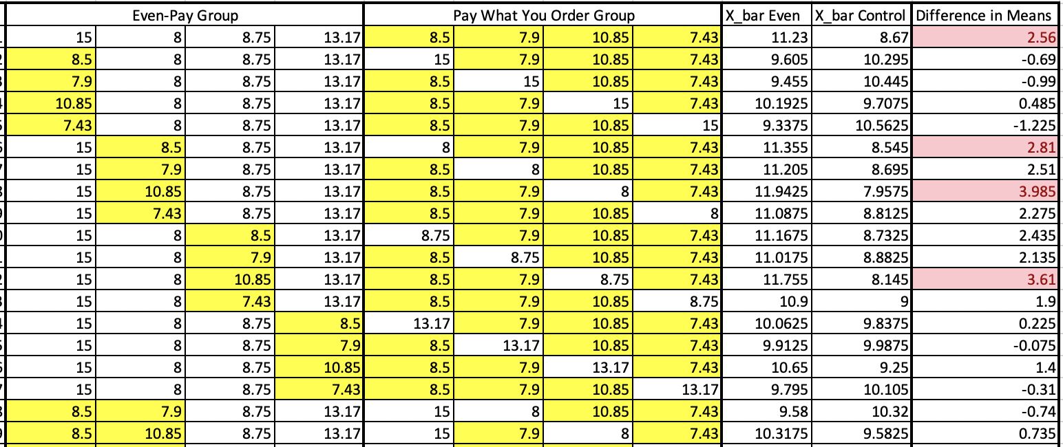
If people order the same amount of food no matter how the bill is split (assuming $H_0$ is true), we assume each person would order the same amount of food regardless of the table they were seated at. Splitting by groups based on how the bill is paid is no different than if the eight values were just randomly divided into two groups of four people. If each person would have ordered the same regardless of which table they were seated at, then another possible sample could have been:

Even Split Group	Pay for what you order (control) Group
$\mathbf{\color{dodgerblue}{\$7.43}}$ , $\$8.00$, $\$8.75$, $\$13.17$	$\$8.50$ , $\$7.90$ , $\$10.85$, $\mathbf{\color{dodgerblue}{\$15.00}}$

Question 1a

What would be the test statistic for the two samples above?

Solution to Question 1a

# find the test statistic for another possible sample

Question 1b

How many different ways can we divide the eight participants into two groups of four?

Solution to Question 1b

# how many possible ways can we create two groups of 4

Two-Sample Permutation Tests

To perform a two-sample permutation test on data collected from two samples size $m$ and $n$:

Pool the $m+n$ values together.
Draw a permutation resample of size $m$ (size of first sample), without replacement.
Use the remaining $n$ (size of second sample) observations for the other sample.
Calculate the difference in means or another statistic to compares samples.
Repeat the resampling process many times and construct the distribution of test statistics.

The p-value is the proportion of times the randomized statistics are as or more extreme than the observed difference.

Permutation resamples of the Unscrupulous Diners Dilemma Data

Case Study: Melanoma Lesion Thickness

Superficial spreading melanoma — Credit: Braga, Macedo, Pinto, et. al., CC BY 4.0, via Wikimedia Commons

Skin is the largest organ in the human body. In the United States, skin cancer is the most common cancer. Current estimates are that one in five Americans will develop skin cancer in their lifetime³. There are different types of skin cancers, and melanoma is one form of skin cancer that is particularly dangerous if not detected early. However, if a skin lesion is detected early, it can be surgically removed before it spreads, and a patient generally has good long-term outcomes.

The data set melanoma in the boot package contains measurements from a random sample of $205$ patients with malignant melanoma at the University Hospital of Odense in Denmark. Each patient had a skin lesion (or tumor) surgically removed and various attributes of the patient and tumors are recorded. Run the code cell below to load the boot package and summarize the variables in the melanoma data set.

library(boot)
summary(melanoma)

      time          status          sex              age             year     
 Min.   :  10   Min.   :1.00   Min.   :0.0000   Min.   : 4.00   Min.   :1962  
 1st Qu.:1525   1st Qu.:1.00   1st Qu.:0.0000   1st Qu.:42.00   1st Qu.:1968  
 Median :2005   Median :2.00   Median :0.0000   Median :54.00   Median :1970  
 Mean   :2153   Mean   :1.79   Mean   :0.3854   Mean   :52.46   Mean   :1970  
 3rd Qu.:3042   3rd Qu.:2.00   3rd Qu.:1.0000   3rd Qu.:65.00   3rd Qu.:1972  
 Max.   :5565   Max.   :3.00   Max.   :1.0000   Max.   :95.00   Max.   :1977  
   thickness         ulcer      
 Min.   : 0.10   Min.   :0.000  
 1st Qu.: 0.97   1st Qu.:0.000  
 Median : 1.94   Median :0.000  
 Mean   : 2.92   Mean   :0.439  
 3rd Qu.: 3.56   3rd Qu.:1.000  
 Max.   :17.42   Max.   :1.000

Question 2

Based on the summary(melanoma) output, give a possible statistical question that could be analyzed using a hypothesis test. Which variable(s) in the melanoma data set would be involved in your analysis?

Tip

Run ?melanoma to access the help documentation and learn more about the data.

Solution to Question 2

Question 3

Which variables in melanoma are categorical? Are those variables being stored as categorical variables? If so, explain how you can tell. If not, in the code cell below, convert the categorical variables to a factor.

Solution to Question 3

# if needed, convert each categorical variable to a factor

Creating a Pooled Sample

Suppose we want to answer the following question: “Is the mean tumor thickness greater for all people with fatal melanoma compared to the mean tumor thickness for all people that survive melanoma?” The two variables of interest are status and thickness.

status: The patients status at the end of the study. 1 indicates that they had died from melanoma, 2 indicates that they were still alive and 3 indicates that they had died from causes unrelated to their melanoma.
thickness: Tumor thickness in millimeters (mm).

For our study, we are comparing two independent populations:

People that have a melanoma tumor removed and survive. This is status group 2.
People that have a melanoma tumor removed and died from melanoma. This is status group 1.
The people in status group 3 we exclude from this analysis.

Question 4

Answer the questions below to state our hypotheses, organize our data, and calculate a test statistic to help determine whether the mean tumor thickness is greater for all people with fatal melanoma compared to the mean tumor thickness for all people that survive melanoma.

Question 4a

Create side-by-side box plots to display the distribution of tumor thickness for each of the three status groups 1 (died from melanoma), 2 (survived), and 3 (died from other causes).

Solution to Question 4a

Fill in the boxplot() command to answer the question.

boxplot(??)

Question 4b

The function tapply(data, index, function) has three inputs:

The data is the data you want to summarize.
The index is a categorical feature that will split the data into two or more different classes or factors.
The function is some function that you want to apply to the data.

Interpret the output from the code cell below.

# run code and interpret output below
tapply(melanoma$thickness, melanoma$status, length)  # nothing to edit

  1   2   3 
 57 134  14

Solution to Question 4b

Question 4c

We would like to use the data in melanoma to test the if the mean tumor thickness is greater for all people with fatal melanoma compared to the mean tumor thickness for all people that survive melanoma. State the corresponding null and alternative hypotheses for this test. Be sure to state each hypothesis both in words and using mathematical notation.

Solution to Question 4c

$H_0$:
$H_a$:

Question 4d

Using the code cell below, subset the melanoma data to create three different vectors:

The vector died is the thickness values for status group 1.
The vector survived is the thickness values for status group 2.
The vector pooled is the thickness values for both status groups 1 and 2 (excluding group 3).

Note

The logical operator == means “is equal to” while the logical operator != means “is not equal to”.

Note

The option drop = TRUE means the output will be a vector of numerical values as opposed to a data frame that has a variable with the name thickness. For example, if we want to calculate the sample mean for the pooled data:

Since the data is stored as a vector, we use mean(pooled). There are no headers in vectors.
If the data is stored as a data frame, we do need to use headers and have mean(pooled$thickness).

The output of the code cell below are vectors, so we do not use the $var_name convention when referring to the sample data which helps simplify the code a little.

Solution to Question 4d

Replace each of the 9 ?? with an appropriate value or variable name.

died <- subset(melanoma, select = ??, ?? == "??", drop = TRUE)
survived <- subset(melanoma, select = ??, ?? == "??", drop = TRUE)
pooled <- subset(melanoma, select = ??, ?? != "??", drop = TRUE)

Question 4e

Using the vectors died, survived, and pooled from Question 4d, calculate the sample size and the sample mean for each of the samples died, survived, and pooled.

Solution to Question 4e

n.died <- ??  # size of sample of melanoma deaths
n.survived <- ??  # size of sample of survivors
n.pooled <- ??  # size of both samples pooled together
xbar.died <- ??  # mean thickness of sample that died
xbar.survived <- ??  # mean thickness of sample that survived
xbar.pooled <- ??  # mean thickness of pooled sample

# print each result to screen
n.died 
n.survived 
n.pooled 
xbar.died 
xbar.survived 
xbar.pooled

Question 4f

Based on the output in Question 4e, calculate, store, and print the test statistic for this test to the screen.

Solution to Question 4f

test.stat <- ??  # compute test statistic
test.stat  # print test statistic to screen

Constructing a Permutation Distribution

Step 1: Create a Vector of Pooled Data

See the code used to create pooled in Question 4d.

Step 2: Create Resamples for Each Treatment Group

For this step, it is important to note the size of each original sample. From Question 4e we know

The sample died consists of 57 observations.
The sample survived consists of 134 observations.
The pooled sample consists of $57 + 134= 191$ observations.

Create an Index Vector

We first create a vector called index that selects (without replacement) 57 random integers out of the integers $1, 2, \ldots , 191$.

set.seed(3021)  # fix the randomization seeding
index <- sample(191, size = 57, replace = FALSE)  # these are the 57 observations chosen for resample 1

The command head(index) shows the first 6 values in the vector index.

head(index)

[1]  55 164  88 189 171  68

The first index value 55 means observation 55 from the pooled vector is the first thickness value randomly assigned to the died sample. From the code cell below, we see the 55th observation in pooled is a thickness of $0.81$ mm.

pooled[55]

[1] 0.81

The next index value 164 means observation 164 from the pooled vector is the second thickness value randomly assigned to the died sample. From the code cell below, we see the 164th observation in pooled is a thickness of $0.65$ mm.

pooled[164]

[1] 0.65

Use `index` to Select Resample of Group 1

The index vector is a vector of integers that tells us which values in pooled are randomly assigned to the died resample. However, index does not contain the corresponding thicknesses of the selected observations. The vector pooled[index] will contain the tumor thicknesses for all 57 randomly selected observations picked in index.

died.resample <- pooled[index]

Use `-index` to Select the Remaining Values for Resample Group 2

The vector index consists of 57 randomly selected integers out of the integers $1, 2, \ldots , 191$.
The vector -index contains the remaining 134 integers that were not selected for index.
The vector pooled[-index] will contain thicknesses for the remaining 134 observations in resample group 2.

survived.resample <- pooled[-index]

Step 3: Calculate the Test Statistic for the Resamples

Calculate the difference in the sample means between the two resamples.

perm.stat <- mean(died.resample) - mean(survived.resample)
perm.stat

[1] -0.1487287

Step 4: Repeat this Many Times to Construct a Permutation Distribution

In practice, it takes a lot of time and energy (and money) to generate all possible resamples (without any duplicate resamples).
- Instead we’ll generate a lot of resamples rather than all possible resamples.
We’ll use $N=10^5-1=99,\!999$ as the default number of resamples. Why use 99,999 resamples?
- We may not generate the original sample as one of the resamples.
- We want to be sure that we do include the original sample when we calculate the p-value.
- We will add the original sample back in with the $99,\!999$ resamples giving $100,\!000$ samples.
The resulting distribution of test statistics of the permutation resamples is called a permutation distribution.
We use the permutation distribution as an estimate for the null distribution to compute the p-value.

Question 5

Complete the first code cell below to create a permutation distribution for the difference in sample mean tumor thickness. Be sure you have already created the vector pooled in Question 4d and stored test.stat in Question 4f.

After generating a permutation distribution, run the second code cell below to create a histogram to display the distribution of resample statistics along with a red vertical line through the observed test statistic. There is nothing to edit in the second code cell.

Solution to Question 5

##########################################
# save all 99,999 permutation resample 
# statistics to the vector perm.stat
##########################################
N <- 10^5 - 1
perm.stat <- numeric(N)

for (i in 1:N)
{
  index <- sample(??, size = ??, replace = ??)  # create index vector
  x.died <- ??  # use index to select died resample
  x.survived <- ??  # the rest of the values go to survived resample
  perm.stat[i] <- ??  # calc difference in sample means
}

##################################################
# plot permutation distribution as a histogram
# mark observed test stat with red vertical line
##################################################
hist(perm.stat, xlab = "xbar.died - xbar.survived",
     main = "Permutation Distribution")
abline(v = test.stat, col = "red")

p-values with Permutation Distributions

We use the permutation distribution as an estimate for the null distribution. The p-value is the proportion of all resampled test statistics that are as or more extreme than the observed test statistic. We can use a logical test to help compute this proportion.

Question 6

How likely is it to get resamples with a difference in means as or more extreme than the observed test statistic? Explain what the code below is doing in practical terms.

p.value <- sum(perm.stat >= test.stat)/N
p.value

Solution to Question 6

Interpret the code cell above.

Question 7

The calculation from Question 6 used the $N=10^5-1=99,\!999$ permutation resamples, but recall we want to be sure to include the original, observed sample when computing the p-value. Explain how the code cell below accomplishes this goal.

p.value <- (sum(perm.stat >= test.stat) + 1) / (N + 1)
p.value

Solution to Question 7

Question 8

Interpret the practical meaning of the p-value from Question 7 to a person who is not very familiar with statistics.

Solution to Question 8

Permutation Test for a Difference in Variances

Question 9

Ulceration is a breakdown of the skin over the melanoma tumor. Using the data set melanoma from the boot package, perform a permutation test to see if the variance of the tumor thickness for ulcerated tumors is different from the variance of the tumor thickness for non-ulcerated tumors.

Tip

The variable ulcer indicates whether the removed tumor was ulcerated (ulcer group 1) or not ulcerated (ulcer group 0).

Question 9a

Write out the null and alternative hypotheses using appropriate notation.

Solution to Question 9a

$H_0$:
$H_a$:

Question 9b

What can we use as the test statistic? What is the value of the observed test statistic?

Solution to Question 9b

test.stat2 <- ??  # compute observed test statistic
test.stat2  # print output to screen

Question 9c

Create a permutation distribution for the difference in sample variances.

Solution to Question 9c

# nothing to edit in this cell
pooled2 <- melanoma$thickness  # create pooled vector of all tumor thicknesses

# Save resamples to vector called result
N <- 10^5 - 1
result <- numeric(N)

# Create permutation distribution
for (i in 1:N)
{
  index <- sample(??, size = ??, replace = ??)
  result[i] <- ??
}

# Display permutation distribution and observed sample diff
hist(result, xlab = "diff in sample variances",
     main = "Permutation Distribution")
abline(v = c(-test.stat2, test.stat2), col = c("blue", "red"))

Question 9d

Calculate the p-value of the observed test statistic and interpret its meaning in practical terms.

Solution to Question 9d

# compute the p-value

Permutation Test for a Difference in Proportions

Question 10

Is the proportion of females with ulcerated tumors less than the proportion of males with ulcerated tumors?

Question 10a

Write out the null and alternative hypotheses using appropriate notation.

Solution to Question 10a

$H_0$:
$H_a$:

Question 10b

What can we use as the test statistic? What is the value of the observed test statistic?

Solution to Question 10b

# original ulceration data for female sample
female <- subset(melanoma, select = "ulcer", sex == "0", drop = TRUE)

# original ulceration data for male sample
male <- subset(melanoma, select = "ulcer", sex == "1", drop = TRUE)

# original ulceration data for both samples pooled together
pooled.sex <- melanoma$ulcer 


# enter a formula to compute the test statistic
test.diff.prop <- ??

Question 10c

Create a permutation distribution for the difference in sample proportions.

Solution to Question 10c

Complete the code cell below.

N <- 10^5 - 1
result.prop <- numeric(N)

for (i in 1:N)
{
  index <- sample(??, size = ??, replace = ??)
  result.prop[i] <- ??
}

hist(result.prop, xlab = "phat1-phat2",
     main = "Permutation Distribution")
abline(v = test.diff.prop, col = "red")

Question 10d

Calculate the p-value of the observed test statistic and interpret its meaning in practical terms.

Solution to Question 10d

# compute the p-value

Permutation Test for Matched Pairs

Question 11

In this example, we use data collected from a matched pair designed study to determine whether smoking during pregnancy is associated with lower birth weight. In our study, we solicit volunteers that have already given birth to two babies. During one of the pregnancies, the parent smoked. During the other pregnancy, they did not smoke. Below is hypothetical data from such a study. A sample of $n=10$ people volunteer to share their data with the researchers from which we have 10 different pairs of birth weights (in grams) summarized in the table below.

	1	2	3	4	5	6	7	8	9	10
No Smoking	2750	2920	3860	3402	2282	3790	3586	3487	2920	2835
Smoked	1790	2381	3940	3317	2125	2665	3572	3156	2721	2225

Question 11a

Researchers are testing to see if the birth weight of babies born to a parent that smoked while pregnant is less, on average, compared to a babies whose parent did not smoke while they were pregnant. Write out the null and alternative hypotheses using appropriate notation.

Solution to Question 11a

$H_0$:
$H_a$:

Question 11b

What can we use as the test statistic? What is the value of the observed test statistic?

Solution to Question 11b

# data from study
no <- c(2750, 2920, 3860, 3402, 2282, 
        3790, 3586, 3487, 2920, 2835)  # non-smoking births weights

smoker <- c(1790, 2381, 3940, 3317, 2125, 
            2665, 3572, 3156, 2721, 2225)  # matching smoking birth weight

diff <- no - smoker  # differences between matched pairs

# Calculate the observed test statistic
test.match.diff <- ??

Question 11c

When we construct a permutation distribution for the sample mean difference between matched pairs, we want to be sure the resampling we use preserves each pairing.

We do not randomize how the pairs are formed.
Each pair of values should remain paired after resampling.
Instead, we randomly assign values in each pair to the smoker and non-smoker positions.

For example, our original sample of matched pair differences is

	1	2	3	4	5	6	7	8	9	10
No Smoking	2750	2920	3860	3402	2282	3790	3586	3487	2920	2835
Smoked	1790	2381	3940	3317	2125	2665	3572	3156	2721	2225
Difference	960	539	-80	85	157	1125	14	331	199	610

One possible resample is given below.

	1	2	3	4	5	6	7	8	9	10
No Smoking Resample	1790	2920	3860	3317	2282	2665	3586	3487	2920	2835
Smoked Resample	2750	2381	3940	3402	2125	3790	3572	3156	2721	2225
Difference Resample	-960	539	-80	-85	157	-1125	14	331	199	610

To create a permutation distribution for the sample mean difference between matched pairs, we randomly choose a sign (positive or negative) for each observed matched-pair difference. Complete the code cell below to generate a permutation distribution for the sample mean difference between matched pairs.

Solution to Question 11c

Complete and run the code cell below to create a permutation distribution.

N <- 10^5-1
perm.match <-numeric(N)

# for each pair, randomly assign the difference to be positive or negative.
# then calculate the new mean of the paired differences
for (i in 1:N)
{
  sign <-sample(c(-1,1), size = ??, replace = ??) # random choose a sign -1 or 1
  diff.resample <- sign * diff
  perm.match[i] <- ??
}

There is nothing to edit in the code cell below. Run the code cell below to plot the permutation distribution and test statistic.

# create a histogram of the permutation distribution
# and add a vertical line at the observed test statistic
hist(perm.match,  xlab = "xbar-diff",
     main = "Permutation Distribution")
abline(v = test.match.diff, col ="red")

Question 11d

Calculate the p-value of the observed test statistic and interpret its meaning in practical terms.

Solution to Question 11d

# compute the p-value

Question 12

Is there a difference in the price of groceries sold by Target and Walmart? The data set Groceries in the resampledata package contains a sample of $n=24$ different grocery items and a pair prices (price at Target and price at Walmart) advertised on their respective websites on a specific day.

First we load the resampledata package.

library(resampledata)  # load resampledata package

Then we print the first six rows of the Groceries data.
Notice this is matched pairs data!

Warning

If you received an error when running the code cell below, it is possible you do not have the resampledata package installed. From the R console, run the command install.packages("resampledata") to first install the resampledata packaged. Run the library(resampledata) command in the code cell above again. Then try running the code cell below again.

head(Groceries)

                             Product    Size Target Walmart Units UnitType
1            Kellogg NutriGrain Bars  8 bars   2.50    2.78     8     bars
2 Quaker Oats Life Cereal  Original     18oz   3.19    6.01    18       oz
3         General Mills Lucky Charms 11.50oz   3.19    2.98    11       oz
4          Quaker Oats Old Fashioned    18oz   2.82    2.68    18       oz
5               Nabisco Oreo Cookies  14.3oz   2.99    2.98    14       oz
6                 Nabisco Chips Ahoy    13oz   2.64    1.98    13       oz

Next, we save corresponding Target and Walmart prices to separate vectors target and walmart.
The first six values in each vector are printed to the screen.
Notice the ordering of the values in each vector is very important to preserve.

target <- Groceries$Target
walmart <- Groceries$Walmart
head(target)

[1] 2.50 3.19 3.19 2.82 2.99 2.64

head(walmart)

[1] 2.78 6.01 2.98 2.68 2.98 1.98

Using the sample data stored in target and walmart, answer the questions below to perform a permutation test.

Set up hypotheses to test whether there a difference in the price of groceries sold by Target and Walmart?
What is the observed test statistic?
Create a permutation distribution for the sample mean difference between matched pairs.
Calculate the p-value.
Interpret the meaning of the p-value.

Solution to Question 12

Creative Commons License

Statistical Methods: Exploring the Uncertain by Adam Spiegler is licensed under a Creative Commons Attribution-NonCommercial-ShareAlike 4.0 International License.

Gneezy, U., E. Haruvy, and H. Yafe (2004), “The Inefficiency of Splitting the Bill”, The Economic Journal 114.↩︎
Glance, N., and B. Huberman, “The Dynamics of Social Dilemmas”, Scientific American↩︎
American Academy of Dermatology, Skin Cancer Stats.↩︎

Even Split Group	Pay for what you order (control) Group
\(\$15.00\), \(\$8.00\), \(\$8.75\), \(\$13.17\)	\(\$8.50\) , \(\$7.90\) , \(\$10.85\), \(\$7.43\)
\(\bar{x}_{\rm even} = \$11.23\)	\(\bar{x}_{\rm control} = \$8.67\)

A Summary of Hypothesis Testing

The Null Distribution and p-values

Case Study: The Unscrupulous Diner’s Dilemma

Step 1: State the Hypotheses

Step 2: Collect Sample Data and Define a Test Statistic

Step 3: How Extreme Is the Observed Difference?

Question 1

Question 1a

Solution to Question 1a

Question 1b

Solution to Question 1b

Two-Sample Permutation Tests

Case Study: Melanoma Lesion Thickness

Question 2

Solution to Question 2

Question 3

Solution to Question 3

Creating a Pooled Sample

Question 4

Question 4a

Solution to Question 4a

Question 4b

Solution to Question 4b

Question 4c

Solution to Question 4c

Question 4d

Solution to Question 4d

Question 4e

Solution to Question 4e

Question 4f

Solution to Question 4f

Constructing a Permutation Distribution

Step 1: Create a Vector of Pooled Data

Step 2: Create Resamples for Each Treatment Group

Create an Index Vector

Use index to Select Resample of Group 1

Use -index to Select the Remaining Values for Resample Group 2

Step 3: Calculate the Test Statistic for the Resamples

Step 4: Repeat this Many Times to Construct a Permutation Distribution

Question 5

Solution to Question 5

p-values with Permutation Distributions

Question 6

Solution to Question 6

Question 7

Solution to Question 7

Question 8

Solution to Question 8

Permutation Test for a Difference in Variances

Question 9

Question 9a

Solution to Question 9a

Question 9b

Solution to Question 9b

Question 9c

Solution to Question 9c

Question 9d

Solution to Question 9d

Permutation Test for a Difference in Proportions

Question 10

Question 10a

Solution to Question 10a

Question 10b

Solution to Question 10b

Question 10c

Solution to Question 10c

Question 10d

Solution to Question 10d

Permutation Test for Matched Pairs

Question 11

Question 11a

Solution to Question 11a

Question 11b

Solution to Question 11b

Question 11c

Solution to Question 11c

Question 11d

Solution to Question 11d

Question 12

Solution to Question 12

Use `index` to Select Resample of Group 1

Use `-index` to Select the Remaining Values for Resample Group 2